HISTOGRAM Statement: CAPABILITY Procedure
Creating a Histogram with Specification Limits
Note: See Histogram with Fitted Normal Curve in the SAS/QC Sample Library.
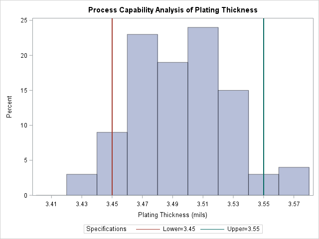
A semiconductor manufacturer produces printed circuit boards that are sampled to determine whether the thickness of their
copper plating lies between a lower specification limit of 3.45 mils and an upper specification limit of 3.55 mils. The plating
process is assumed to be in statistical control. The plating thicknesses of 100 boards are saved in a data set named Trans, created by the following statements:
data Trans;
   input Thick @@;
   label Thick='Plating Thickness (mils)';
   datalines;
3.468 3.428 3.509 3.516 3.461 3.492 3.478 3.556 3.482 3.512
3.490 3.467 3.498 3.519 3.504 3.469 3.497 3.495 3.518 3.523
3.458 3.478 3.443 3.500 3.449 3.525 3.461 3.489 3.514 3.470
3.561 3.506 3.444 3.479 3.524 3.531 3.501 3.495 3.443 3.458
3.481 3.497 3.461 3.513 3.528 3.496 3.533 3.450 3.516 3.476
3.512 3.550 3.441 3.541 3.569 3.531 3.468 3.564 3.522 3.520
3.505 3.523 3.475 3.470 3.457 3.536 3.528 3.477 3.536 3.491
3.510 3.461 3.431 3.502 3.491 3.506 3.439 3.513 3.496 3.539
3.469 3.481 3.515 3.535 3.460 3.575 3.488 3.515 3.484 3.482
3.517 3.483 3.467 3.467 3.502 3.471 3.516 3.474 3.500 3.466
;
The following statements create the histogram shown in Figure 5.8:
title 'Process Capability Analysis of Plating Thickness';
proc capability data=Trans noprint;
   spec lsl = 3.45 usl = 3.55;
   histogram Thick / odstitle = title;
run;
A histogram is created for each variable listed after the keyword HISTOGRAM. The SPEC statement, which is optional, provides the specification limits that are displayed on the histogram. For more information about the SPEC statement, see SPEC Statement.
The NOPRINT
option suppresses printed output with summary statistics for the variable Thick that would be displayed by default. See Computing Descriptive Statistics for an example of this output.
Figure 5.8: Histogram Created with Traditional Graphics

