The UNIVARIATE Procedure
- Overview
-
Getting Started

-
Syntax
-
DetailsMissing ValuesRoundingDescriptive StatisticsCalculating the ModeCalculating PercentilesTests for LocationConfidence Limits for Parameters of the Normal DistributionRobust EstimatorsCreating Line Printer PlotsCreating High-Resolution GraphicsUsing the CLASS Statement to Create Comparative PlotsPositioning InsetsFormulas for Fitted Continuous DistributionsGoodness-of-Fit TestsKernel Density EstimatesConstruction of Quantile-Quantile and Probability PlotsInterpretation of Quantile-Quantile and Probability PlotsDistributions for Probability and Q-Q PlotsEstimating Shape Parameters Using Q-Q PlotsEstimating Location and Scale Parameters Using Q-Q PlotsEstimating Percentiles Using Q-Q PlotsInput Data SetsOUT= Output Data Set in the OUTPUT StatementOUTHISTOGRAM= Output Data SetOUTKERNEL= Output Data SetOUTTABLE= Output Data SetTables for Summary StatisticsODS Table NamesODS Tables for Fitted DistributionsODS GraphicsComputational Resources
-
ExamplesComputing Descriptive Statistics for Multiple VariablesCalculating ModesIdentifying Extreme Observations and Extreme ValuesCreating a Frequency TableCreating Plots for Line Printer OutputAnalyzing a Data Set With a FREQ VariableSaving Summary Statistics in an OUT= Output Data SetSaving Percentiles in an Output Data SetComputing Confidence Limits for the Mean, Standard Deviation, and VarianceComputing Confidence Limits for Quantiles and PercentilesComputing Robust EstimatesTesting for LocationPerforming a Sign Test Using Paired DataCreating a HistogramCreating a One-Way Comparative HistogramCreating a Two-Way Comparative HistogramAdding Insets with Descriptive StatisticsBinning a HistogramAdding a Normal Curve to a HistogramAdding Fitted Normal Curves to a Comparative HistogramFitting a Beta CurveFitting Lognormal, Weibull, and Gamma CurvesComputing Kernel Density EstimatesFitting a Three-Parameter Lognormal CurveAnnotating a Folded Normal CurveCreating Lognormal Probability PlotsCreating a Histogram to Display Lognormal FitCreating a Normal Quantile PlotAdding a Distribution Reference LineInterpreting a Normal Quantile PlotEstimating Three Parameters from Lognormal Quantile PlotsEstimating Percentiles from Lognormal Quantile PlotsEstimating Parameters from Lognormal Quantile PlotsComparing Weibull Quantile PlotsCreating a Cumulative Distribution PlotCreating a P-P Plot
- References
Exploring a Data Distribution
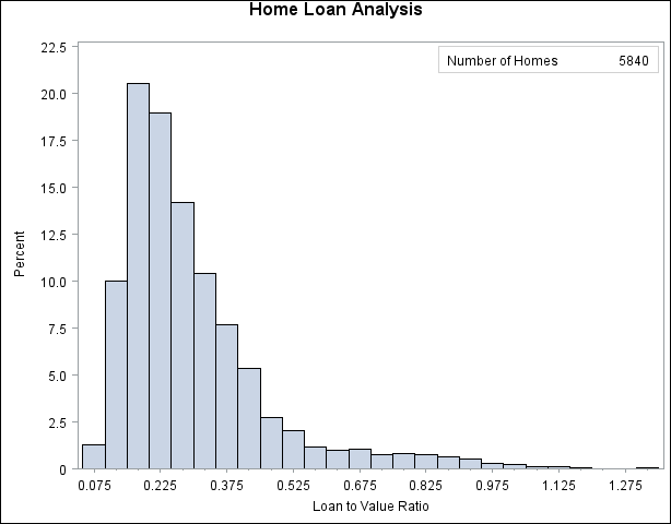
Figure 4.2 shows a histogram of the loan-to-value ratios. The histogram reveals features of the ratio distribution, such as its skewness and the peak at 0.175, which are not evident from the tables in the previous example. The following statements create the histogram:
ods graphics off;
title 'Home Loan Analysis';
proc univariate data=HomeLoans noprint;
   histogram LoanToValueRatio;
   inset n = 'Number of Homes' / position=ne;
run;
By default, PROC UNIVARIATE produces traditional graphics output, and the basic appearance of the histogram is determined by the prevailing ODS style. The NOPRINT option suppresses the display of summary statistics. The INSET statement inserts the total number of analyzed home loans in the upper right (northeast) corner of the plot.
Figure 4.2: Histogram for Loan-to-Value Ratio
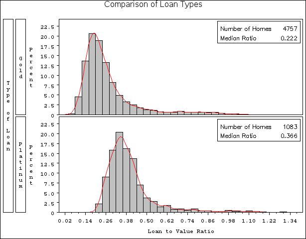
The data set HomeLoans contains a variable named LoanType that classifies the loans into two types: Gold and Platinum. It is useful to compare the distributions of LoanToValueRatio for the two types. The following statements request quantiles for each distribution and a comparative histogram, which are
shown in Figure 4.3 and Figure 4.4.
title 'Comparison of Loan Types';
options nogstyle;
ods select Quantiles MyHist;
proc univariate data=HomeLoans;
   var LoanToValueRatio;
   class LoanType;
   histogram LoanToValueRatio / kernel(color=red)
                                cfill=ltgray
                                name='MyHist';
   inset n='Number of Homes' median='Median Ratio' (5.3) / position=ne;
   label LoanType = 'Type of Loan';
run;
options gstyle;
The ODS SELECT statement restricts the default output to the tables of quantiles and the graph produced by the HISTOGRAM statement,
which is identified by the value specified by the NAME= option. The CLASS statement specifies LoanType as a classification variable for the quantile computations and comparative histogram. The KERNEL option adds a smooth nonparametric
estimate of the ratio density to each histogram. The INSET statement specifies summary statistics to be displayed directly
in the graph.
The NOGSTYLE system option specifies that the ODS style not influence the appearance of the histogram. Instead, the CFILL= option determines the color of the histogram bars and the COLOR= option specifies the color of the kernel density curve.
Figure 4.3: Quantiles for Loan-to-Value Ratio
| Comparison of Loan Types |
| Quantiles (Definition 5) | |
|---|---|
| Quantile | Estimate |
| 100% Max | 1.0617647 |
| 99% | 0.8974576 |
| 95% | 0.6385908 |
| 90% | 0.4471369 |
| 75% Q3 | 0.2985099 |
| 50% Median | 0.2217033 |
| 25% Q1 | 0.1734568 |
| 10% | 0.1411130 |
| 5% | 0.1213079 |
| 1% | 0.0942167 |
| 0% Min | 0.0651786 |
| Comparison of Loan Types |
| Quantiles (Definition 5) | |
|---|---|
| Quantile | Estimate |
| 100% Max | 1.312981 |
| 99% | 1.050000 |
| 95% | 0.691803 |
| 90% | 0.549273 |
| 75% Q3 | 0.430160 |
| 50% Median | 0.366168 |
| 25% Q1 | 0.314452 |
| 10% | 0.273670 |
| 5% | 0.253124 |
| 1% | 0.231114 |
| 0% Min | 0.215504 |
The output in Figure 4.3 shows that the median ratio for Platinum loans (0.366) is greater than the median ratio for Gold loans (0.222). The comparative histogram in Figure 4.4 enables you to compare the two distributions more easily. It shows that the ratio distributions are similar except for a shift of about 0.14.
Figure 4.4: Comparative Histogram for Loan-to-Value Ratio
A sample program for this example, univar1.sas, is available in the SAS Sample Library for Base SAS software.