Example 4.28 Creating a Normal Quantile Plot

This example illustrates how to create a normal quantile plot. An engineer is analyzing the distribution of distances between holes cut in steel sheets. The following statements save measurements of the distance between two holes cut into 50 steel sheets as values of the variable Distance in the data set Sheets:

data Sheets;
   input Distance @@;
   label Distance = 'Hole Distance (cm)';
   datalines;
 9.80 10.20 10.27  9.70  9.76
10.11 10.24 10.20 10.24  9.63
 9.99  9.78 10.10 10.21 10.00
 9.96  9.79 10.08  9.79 10.06
10.10  9.95  9.84 10.11  9.93
10.56 10.47  9.42 10.44 10.16
10.11 10.36  9.94  9.77  9.36
 9.89  9.62 10.05  9.72  9.82
 9.99 10.16 10.58 10.70  9.54
10.31 10.07 10.33  9.98 10.15
;
run;

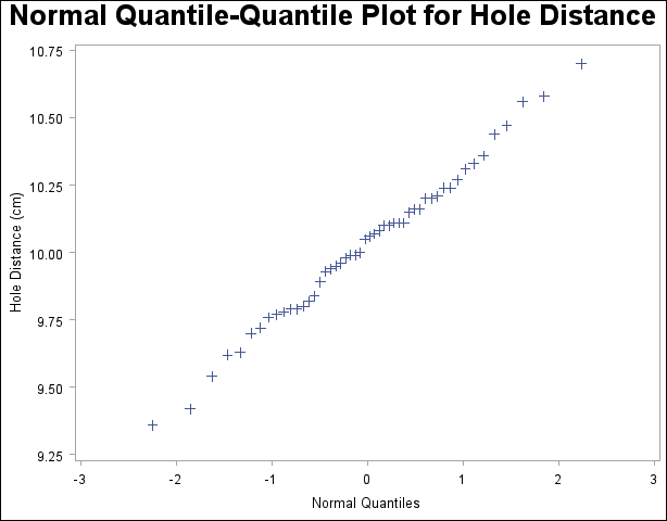
The engineer decides to check whether the distribution of distances is normal. The following statements create a Q-Q plot for Distance, shown in Output 4.28.1:

symbol v=plus;
title 'Normal Quantile-Quantile Plot for Hole Distance';
proc univariate data=Sheets noprint;
   qqplot Distance;
run;

The plot compares the ordered values of Distance with quantiles of the normal distribution. The linearity of the point pattern indicates that the measurements are normally distributed. Note that a normal Q-Q plot is created by default.

Output 4.28.1 Normal Quantile-Quantile Plot for Distance

A sample program for this example, uniex17.sas, is available in the SAS Sample Library for Base SAS software.