| The UNIVARIATE Procedure |
Example 4.27 Creating a Histogram to Display Lognormal Fit
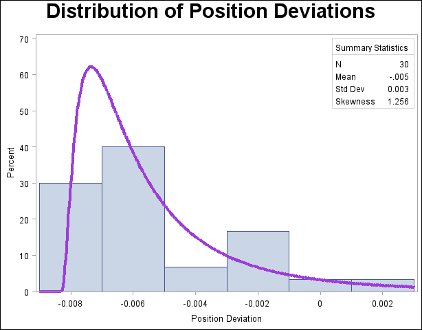
This example uses the data set Aircraft from Example 4.26 to illustrate how to display a lognormal fit with a histogram. To determine whether the lognormal distribution is an appropriate model for a distribution, you should consider the graphical fit as well as conduct goodness-of-fit tests. The following statements fit a lognormal distribution and display the density curve on a histogram:
title 'Distribution of Position Deviations';
ods select Lognormal.ParameterEstimates Lognormal.GoodnessOfFit MyPlot;
proc univariate data=Aircraft;
   var Deviation;
   histogram / lognormal(w=3 theta=est)
               vaxis = axis1
               name  = 'MyPlot';
   inset n mean (5.3) std='Std Dev' (5.3) skewness (5.3) /
         pos = ne  header = 'Summary Statistics';
   axis1 label=(a=90 r=0);
run;
The ODS SELECT statement restricts the output to the "ParameterEstimates" and "GoodnessOfFit" tables; see the section ODS Table Names. The LOGNORMAL primary option superimposes a fitted curve on the histogram in Output 4.27.1. The W= option specifies the line width for the curve. The INSET statement specifies that the mean, standard deviation, and skewness be displayed in an inset in the northeast corner of the plot. Note that the default value of the threshold parameter  is zero. In applications where the threshold is not zero, you can specify
  with the THETA= option. The variable Deviation includes values that are less than the default threshold; therefore, the option THETA= EST is used.

Output 4.27.2 provides three EDF goodness-of-fit tests for the lognormal distribution: the Anderson-Darling, the Cramér-von Mises, and the Kolmogorov-Smirnov tests. The null hypothesis for the three tests is that a lognormal distribution holds for the sample data.
| Parameters for Lognormal Distribution | ||
|---|---|---|
| Parameter | Symbol | Estimate |
| Threshold | Theta | -0.00834 |
| Scale | Zeta | -6.14382 |
| Shape | Sigma | 0.882225 |
| Mean | -0.00517 | |
| Std Dev | 0.003438 | |
The  -values for all three tests are greater than 0.5, so the null hypothesis is not rejected. The tests support the conclusion that the two-parameter lognormal distribution with scale parameter
  and shape parameter
  provides a good model for the distribution of position deviations. For further discussion of goodness-of-fit interpretation, see the section Goodness-of-Fit Tests.
A sample program for this example, uniex16.sas, is available in the SAS Sample Library for Base SAS software.
Copyright © SAS Institute, Inc. All Rights Reserved.