Wavelet Analysis

You can use the WAVIFT subroutine to invert a wavelet transformation computed with the WAVFT subroutine. If no thresholding is specified, then up to numerical rounding error this inversion is exact. The following statements provide an illustration of this:

 
      call wavift(reconstructedAbsorbance,decomp); 
      errorSS=ssq(absorbance-reconstructedAbsorbance); 
      print "The reconstruction error sum of squares = " errorSS; 

The output is shown in Figure 20.15.

Usually you use the WAVIFT subroutine with thresholding specified. This yields a smoothed reconstruction of the input data. You can use the following statements to create a smoothed reconstruction of absorbance and add this variable to the QuartzInfraredSpectrum data set.

 
      call wavift(smoothedAbsorbance,decomp,&SureShrink); 
      create temp from smoothedAbsorbance[colname='smoothedAbsorbance']; 
         append from smoothedAbsorbance; 
      close temp; 
   quit; 

   data quartzInfraredSpectrum;   
     set quartzInfraredSpectrum; 
     set temp; 
   run; 

The following statements produce the line plot of the smoothed absorbance data shown in Figure 20.16:

 
   symbol1 c=black i=join v=none;    
   proc gplot data=quartzInfraredSpectrum; 
      plot smoothedAbsorbance*WaveNumber/ 
           hminor = 0   vminor = 0 
           vaxis  = axis1 
           hreverse frame; 
           axis1 label = ( r=0 a=90 ); 
   run; 

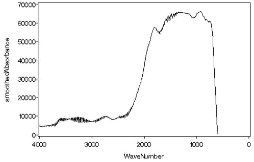
You can see by comparing Figure 20.1 with Figure 20.16 that the wavelet smooth of the absorbance data has preserved all the essential features of these data.