Time Series Analysis and Examples: Smoothness Priors Modeling

Time Series Analysis and Examples

Smoothness Priors Modeling

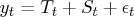
Consider the time series :

$y_t = f(t) + \epsilon_t$

where

is an unknown smooth function and $\epsilon_t$ is an

random variable with zero mean and positive variance $\sigma^2$ . Whittaker (1923) provides the solution, which balances a tradeoff between closeness to the data and the

th-order difference equation. For a fixed value of $\lambda$ and

, the solution $\hat{f}$ satisfies

$\min_f \sum_{t=1}^t \{ [y_t - f(t)]^2 + \lambda^2 [\nabla^k f(t)]^2 \}$

where $\nabla^k$ denotes the

th-order difference operator. The value of $\lambda$ can be viewed as the smoothness tradeoff measure. Akaike (1980a) proposed the Bayesian posterior PDF to solve this problem.

$\ell(f) = \exp \{ -\frac{1}{2 \sigma^2} \sum_{t=1}^t [y_t - f(t)]^2 \} \exp \{ -\frac{\lambda^2}{2 \sigma^2} \sum_{t=1}^t [\nabla^k f(t)]^2 \}$

Therefore, the solution can be obtained when the function $\ell(f)$ is maximized.

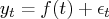
Assume that time series is decomposed as follows:

$y_t = t_t + s_t + \epsilon_t$

where

denotes the trend component and

is the seasonal component. The trend component follows the

th-order stochastically perturbed difference equation.

$\nabla^k t_t = w_{1t}, \hspace*{0.25in} w_{1t} \sim n(0,\tau_1^2)$

For example, the polynomial trend component for

is written as

$t_t = 2t_{t-1} - t_{t-2} + w_{1t}$

To accommodate regular seasonal effects, the stochastic seasonal relationship is used.

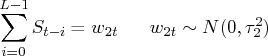
$\sum_{i=0}^{l-1} s_{t-i} = w_{2t} \hspace*{0.25in} w_{2t} \sim n(0,\tau_2^2)$

where

is the number of seasons within a period. In the context of Whittaker and Akaike, the smoothness priors problem can be solved by the maximization of

$\ell(f) & = & \exp [ -\frac{1}{2 \sigma^2} \sum_{t=1}^t (y_t - t_t - s_t)^2 ... ...\frac{\tau_2^2}{2 \sigma^2} \sum_{t=1}^t ( \sum_{i=0}^{l-1} s_{t-i} )^2 ]$

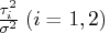
The values of hyperparameters $\tau_1^2$ and $\tau_2^2$ refer to a measure of uncertainty of prior information. For example, the large value of $\tau_1^2$ implies a relatively smooth trend component. The ratio $\frac{\tau_i^2}{\sigma^2}\; (i=1,2)$ can be considered as a signal-to-noise ratio.

Kitagawa and Gersch (1984) use the Kalman filter recursive computation for the likelihood of the tradeoff parameters. The hyperparameters are estimated by combining the grid search and optimization method. The state space model and Kalman filter recursive computation are discussed in the section "State Space and Kalman Filter Method".

Top of Page