GCONTOUR Procedure

Example 4: Using Patterns and Joins

Features:	PLOT statement options: COUTLINE= CTEXT= HAXIS= JOIN LEGEND= PATTERN VAXIS=
Other features:	AXIS statement options: COLOR= LABEL= VALUE= WIDTH= LEGEND statement
Data set:	SWIRL
Sample library member:	GCTPATJ

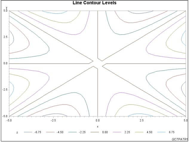
This example demonstrates the differences between using lines and patterns to represent contour levels. The first PLOT statement generates a plot with lines representing contour levels.

Line Contour Levels

The second PLOT statement specifies the PATTERN option to fill and color contour levels. Additional PLOT statement options outline filled areas in gray and specify green text for all text on the axes and in the legend.

Pattern Contour Levels

The third PLOT statement uses the JOIN option to combine adjacent grid cells with the same pattern to form a single pattern area. Additional options enhance the plot by modifying the axes and framing the legend.

Contour Plot with Joined Cells

Program

goptions reset=all border;

data swirl; 
    do x= -5 to 5 by 0.25;
       do y= -5 to 5 by 0.25;
          if x+y=0 then z=0;
             else z=(x*y)*((x*x-y*y)/(x*x+y*y)); 
          output; 
       end; 
    end; 
run;

title1 "Line Contour Levels";
footnote1 j=r "GCTPATR1";

proc gcontour data=swirl;
   plot y*x=z;
run;
quit;

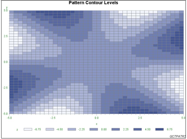
title1 "Pattern Contour Levels";
footnote j=r "GCTPATR2";

proc gcontour data=swirl;
   plot y*x=z / 
      ctext=green
      coutline=gray
      pattern;
run;
quit;

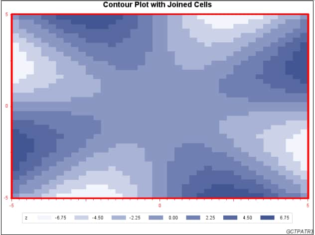
title "Contour Plot with Joined Cells";
footnote j=r "GCTPATR3";

axis1 label=none 
    value=("-5" '' "0" '' "5")
    color=red 
     width=3;
  axis2 label=none 
     value=("-5" '' "0" '' "5")
     color=red  
     width=3;

legend1 frame;

proc gcontour data=swirl;
    plot y*x=z / 
        haxis=axis1
       join
       legend=legend1
       pattern
       vaxis=axis2;
run;
quit;

Program Description

Set the graphics environment. Draw a border around the graphics output area.

goptions reset=all border;

Create the data set. The data set SWIRL is generated data that produces a symmetric contour pattern, which is useful for illustrating the pattern option.

data swirl; 
    do x= -5 to 5 by 0.25;
       do y= -5 to 5 by 0.25;
          if x+y=0 then z=0;
             else z=(x*y)*((x*x-y*y)/(x*x+y*y)); 
          output; 
       end; 
    end; 
run;

Define the title and the footnote. Add TITLE content. Add FOOTNOTE content, and placement.

title1 "Line Contour Levels";
footnote1 j=r "GCTPATR1";

Generate the first contour plot. Generate a simple contour plot.

proc gcontour data=swirl;
   plot y*x=z;
run;
quit;

Define the title and footnote for the second plot. Add TITLE content for the second plot. Add FOOTNOTE content and placement for the second plot.

title1 "Pattern Contour Levels";
footnote j=r "GCTPATR2";

Generate the second contour plot. CTEXT=green specifies green for all text on the axes and legend. COUTLINE=gray specifies gray outlining of filled areas. The PATTERN option specifies the fill pattern and colors for the contour levels.

proc gcontour data=swirl;
   plot y*x=z / 
      ctext=green
      coutline=gray
      pattern;
run;
quit;

Define the title and footnote for the third plot. Add TITLE content for the third plot. Add FOOTNOTE content and placement for the third plot.

title "Contour Plot with Joined Cells";
footnote j=r "GCTPATR3";

Define the axis characteristics. Blanks are used to suppress tick mark labels at positions -2.5 and 2.5.

axis1 label=none 
    value=("-5" '' "0" '' "5")
    color=red 
     width=3;
  axis2 label=none 
     value=("-5" '' "0" '' "5")
     color=red  
     width=3;

Define the legend characteristics. Add a frame around the legend.

legend1 frame;

Generate the third contour plot. The HAXIS=AXIS1 option assigns an axis definition to the horizontal axis. The JOIN= option combines adjacent grid cells with the same pattern to form a single pattern area. LEGEND=LEGEND1 assigns the legend definition. The PATTERN option specifies the fill pattern and colors for the contour levels. VAXIS=AXIS2 assigns an axis definition to the vertical axis.

proc gcontour data=swirl;
    plot y*x=z / 
        haxis=axis1
       join
       legend=legend1
       pattern
       vaxis=axis2;
run;
quit;