G3GRID Procedure

Interpolation Methods

Types of Interpolation Methods

The G3GRID procedure can use one of three interpolation methods: bivariate interpolation (the default), spline interpolation, and smoothing spline interpolation.

Bivariate Interpolation

Unless you specify the SPLINE option, the G3GRID procedure is an interpolation procedure. It calculates the z values for x, y points that are missing from the input data set. The surface that is formed by the interpolated data passes precisely through the data points in the input data set.

This method of interpolation works best for fairly smooth functions, with values given at uniformly distributed points in the plane. If the data points in the input data set are erratic, the default interpolated surface can be erratic.

This default method is a modification of that described by Akima (1978). This method consists of the following actions:

dividing the plane into non-overlapping triangles that use the positions of the available points
fitting a bivariate fifth degree polynomial within each triangle
calculating the interpolated values by evaluating the polynomial at each grid point that falls in the triangle

The coefficients for the polynomial are computed based on the following criteria:

the values of the function at the vertices of the triangle
the estimated values for the first, and second derivatives of the function at the vertices

The estimates of the first, and second derivatives are computed using the n nearest neighbors of the point, where n is the number specified in the GRID statement's NEAR= option. A Delauney triangulation (Ripley 1981, p. 38), is used for the default method. The coordinates of the triangles are available in an output data set, if requested by the OUTTRI= option, in the PROC G3GRID statement. This is the default interpolation method.

Spline Interpolation

If you specify the SPLINE option, a method is used that produces either an interpolation. or smoothing that is optimally smooth. See (Harder and Desmarais 1972, Meinguet 1979, Green and Silverman 1994). The surface that is generated can be thought of as one that would be formed if a stiff, thin metal plate were forced through, or near the given data points. For large data sets, this method is substantially more expensive than the default method.

The function u, formed when you specify the SPLINE option, is determined by letting:

and

where

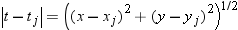
The coefficients c₁, c₂,..., c_n, andd₁, d₂, d₃ of this polynomial are determined by the following equations:

and

where

is the n × n matrix E(t_i, t_j )

is the n × n identity matrix

is the smoothing parameter that is specified in the SMOOTH= option

is (c₁ ,..., c_n )

is (z₁ ,..., z_n )

is (d₁, d₂, d₃)

is the n × three matrix whose ith row is (1, x_i, y_i).

See Wahba (1990) for more detail.

Spline Smoothing

Using the SMOOTH= option in the GRID statement with the SPLINE option, enables you to produce a smoothing spline. See Eubank (1988) for a general discussion of spline smoothing. The value or values specified in the SMOOTH= option are substituted for λ in the equation that is described in Spline Interpolation. A smoothing spline trades closeness to the original data points for smoothness. To find a value that produces the best balance between smoothness, and fit to the original data, several values for the SMOOTH= option can be run.