The SIMLIN Procedure

Example 32.2 Multipliers for a Third-Order System
This example shows how to fit and simulate a single equation dynamic model with third-order lags. It then shows how to convert the third-order equation into a three equation system with only first-order lags, so that the SIMLIN procedure can compute multipliers. (See the section "Multipliers for Higher Order Lags" earlier in this chapter for more information.)
The input data set TEST is created from simulated data. A partial listing of the data set TEST produced by PROC PRINT is shown in Output 32.2.1.
Output 32.2.1: Partial Listing of Input Data Set
| Simulate Equation with Third-Order Lags |
| Listing of Simulated Input Data |
| Obs | y | ylag1 | ylag2 | ylag3 | x | n |
|---|---|---|---|---|---|---|
| 1 | 8.2369 | 8.5191 | 6.9491 | 7.8800 | -1.2593 | 1 |
| 2 | 8.6285 | 8.2369 | 8.5191 | 6.9491 | -1.6805 | 2 |
| 3 | 10.2223 | 8.6285 | 8.2369 | 8.5191 | -1.9844 | 3 |
| 4 | 10.1372 | 10.2223 | 8.6285 | 8.2369 | -1.7855 | 4 |
| 5 | 10.0360 | 10.1372 | 10.2223 | 8.6285 | -1.8092 | 5 |
| 6 | 10.3560 | 10.0360 | 10.1372 | 10.2223 | -1.3921 | 6 |
| 7 | 11.4835 | 10.3560 | 10.0360 | 10.1372 | -2.0987 | 7 |
| 8 | 10.8508 | 11.4835 | 10.3560 | 10.0360 | -1.8788 | 8 |
| 9 | 11.2684 | 10.8508 | 11.4835 | 10.3560 | -1.7154 | 9 |
| 10 | 12.6310 | 11.2684 | 10.8508 | 11.4835 | -1.8418 | 10 |
The REG procedure processes the input data and writes the parameter estimates to the OUTEST= data set A.
title2 'Estimated Parameters';
proc reg data=test outest=a;
   model y=ylag3 x;
run;

title2 'Listing of OUTEST= Data Set';
proc print data=a;
run;
Output 32.2.2 shows the printed output produced by the REG procedure, and Output 32.2.3 displays the OUTEST= data set A produced.
Output 32.2.2: Estimates and Fit Information from PROC REG
Output 32.2.3: The OUTEST= Data Set Created by PROC REG
The SIMLIN procedure processes the TEST data set using the estimates from PROC REG. The following statements perform the simulation and write the results to the OUT= data set OUT2.
title2 'Simulation of Equation';
proc simlin est=a data=test nored;
   endogenous y;
   exogenous  x;
   lagged ylag3 y 3;
   id n;
   output out=out1 predicted=yhat residual=yresid;
run;
The printed output from the SIMLIN procedure is shown in Output 32.2.4.
Output 32.2.4: Output Produced by PROC SIMLIN
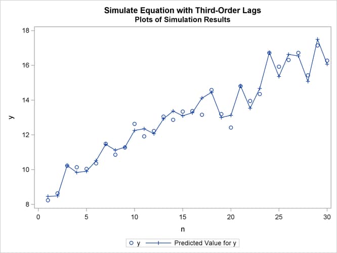
The following statements plot the actual and predicted values, as shown in Output 32.2.5.
title2 'Plots of Simulation Results';
proc sgplot data=out1;
   scatter x=n y=y;
   series x=n y=yhat / markers markerattrs=(symbol=plus);
run;
Output 32.2.5: Plot of Predicted and Actual Values
Next, the input data set TEST is modified by creating two new variables, YLAG1X and YLAG2X, that are equal to YLAG1 and YLAG2. These variables are used in the SYSLIN procedure. (The estimates produced by PROC SYSLIN are the same as before and are not shown.) A listing of the OUTEST= data set B created by PROC SYSLIN is shown in Output 32.2.6.
data test2;
   set test;
   ylag1x=ylag1;
   ylag2x=ylag2;
run;
title2 'Estimation of parameters and definition of identities';
proc syslin data=test2 outest=b;
   endogenous y ylag1x ylag2x;
   model y=ylag3 x;
   identity ylag1x=ylag1;
   identity ylag2x=ylag2;
run;

title2 'Listing of OUTEST= data set from PROC SYSLIN';
proc print data=b;
run;
Output 32.2.6: Listing of OUTEST= Data Set Created from PROC SYSLIN
| Simulate Equation with Third-Order Lags |
| Listing of OUTEST= data set from PROC SYSLIN |
| Obs | _TYPE_ | _STATUS_ | _MODEL_ | _DEPVAR_ | _SIGMA_ | Intercept | ylag3 | x | ylag1 | ylag2 | y | ylag1x | ylag2x |
|---|---|---|---|---|---|---|---|---|---|---|---|---|---|
| 1 | OLS | 0 Converged | y | y | 0.22675 | 0.14239 | 0.77121 | -1.77668 | . | . | -1 | . | . |
| 2 | IDENTITY | 0 Converged | ylag1x | . | 0.00000 | . | . | 1 | . | . | -1 | . | |
| 3 | IDENTITY | 0 Converged | ylag2x | . | 0.00000 | . | . | . | 1 | . | . | -1 |
The SIMLIN procedure is used to compute the reduced form and multipliers. The OUTEST= data set B from PROC SYSLIN is used as the EST= data set for the SIMLIN procedure. The following statements perform the multiplier analysis.
title2 'Simulation of transformed first-order equation system';

proc simlin est=b data=test2 total interim=2;
   endogenous y ylag1x ylag2x;
   exogenous  x;
   lagged  ylag1 y 1  ylag2 ylag1x 1  ylag3 ylag2x 1;
   id n;
   output out=out2 predicted=yhat residual=yresid;
run;
Output 32.2.7 shows the interim 2 and total multipliers printed by the SIMLIN procedure.
Output 32.2.7: Interim 2 and Total Multipliers