The HPCDM Procedure(Experimental)

Example 18.1 Estimating the Probability Distribution of Insurance Payments
The primary outcome of running PROC HPCDM is the estimate of the compound distribution of aggregate loss, given the distributions of frequency and severity of the individual losses. This aggregate loss is often referred to as the ground-up loss. If you are an insurance company or a bank, you are also interested in acting on the ground-up loss by computing an entity that is derived from the ground-up loss. For example, you might want to estimate the distribution of the amount that you are expected to pay for the losses or the distribution of the amount that you can offload onto another organization, such as a reinsurance company. PROC HPCDM enables you to specify a severity adjustment program, which is a sequence of SAS programming statements that adjust the severity of the individual loss event to compute the entity of interest. Your severity adjustment program can use external information that is recorded as variables in the observations of the DATA= data set in addition to placeholder symbols for information that PROC HPCDM generates internally, such as the severity of the current loss event (_SEV_) and the sum of the adjusted severity values of the events that have been simulated thus far for the current sample point (_CUMADJSEV_). If you are doing a scenario analysis such that a scenario contains more than one observation, then you can also access the cumulative severity and cumulative adjusted severity for the current observation by using the _CUMSEVFOROBS_ and _CUMADJSEVFOROBS_ symbols.
This example continues the example of the section Scenario Analysis to illustrate how you can estimate the distribution of the aggregate amount that is paid to a group of policyholders. Let
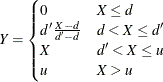
the amount that is paid to an individual policyholder be computed by using what is usually referred to as a disappearing deductible (Klugman, Panjer, and Willmot 1998, Ch. 2). If X denotes the ground-up loss that a policyholder incurs, d denotes the lower limit on the deductible,  denotes the upper limit on the deductible, and u denotes the limit on the total payments that are made to a policyholder in a year, then Y, the amount that is paid to the policyholder for each loss event, is defined as follows:
You can encode this logic by using a set of SAS programming statements.
Extend the Work.GroupOfPolicies data set in the example in the section Scenario Analysis to include the following three additional variables for each policyholder: LowDeductible to record d, HighDeductible to record , and Limit to record u. The data set contains the observations as shown in Output 18.1.1.
Output 18.1.1: Scenario Analysis Data for Multiple Policyholders with Policy Provisions
| policyholderId | age | gender | carType | annualMiles | education | carSafety | income | lowDeductible | highDeductible | limit | annualLimit |
|---|---|---|---|---|---|---|---|---|---|---|---|
| 1 | 1.18 | 2 | 1 | 2.2948 | 3 | 0.99532 | 1.59870 | 400 | 1400 | 7500 | 10000 |
| 2 | 0.66 | 2 | 2 | 2.8148 | 1 | 0.05625 | 0.67539 | 300 | 1300 | 2500 | 20000 |
| 3 | 0.82 | 1 | 2 | 1.6130 | 2 | 0.84146 | 1.05940 | 100 | 1100 | 5000 | 10000 |
| 4 | 0.44 | 1 | 1 | 1.2280 | 3 | 0.14324 | 0.24110 | 300 | 800 | 5000 | 20000 |
| 5 | 0.44 | 1 | 1 | 0.9670 | 2 | 0.08656 | 0.65979 | 100 | 1100 | 5000 | 20000 |
The following PROC HPCDM step estimates the compound distributions of the aggregate loss and the aggregate amount that is
paid to the group of policyholders in the Work.GroupOfPolicies data set by using the count model that is stored in the Work.CountregModel item store and the lognormal severity model that is stored in the Work.SevRegEst data set:
/* Simulate the aggregate loss distribution and aggregate adjusted
   loss distribution for the scenario with multiple policyholders */
proc hpcdm data=groupOfPolicies nreplicates=10000 seed=13579 print=all
           countstore=work.countregmodel severityest=work.sevregest
           plots=(edf pdf) nperturbedSamples=50
           adjustedseverity=amountPaid;
   severitymodel logn;

   if (_sev_ <= lowDeductible) then
      amountPaid = 0;
   else do;
      if (_sev_ <= highDeductible) then
         amountPaid = highDeductible *
            (_sev_-lowDeductible)/(highDeductible-lowDeductible);
      else
         amountPaid = MIN(_sev_, limit); /* imposes per-loss payment limit */
   end;
run;
The preceding step uses a severity adjustment program to compute the value of the symbol AmountPaid and specifies that symbol in the ADJUSTEDSEVERITY= option in the PROC HPCDM step. The program is executed for each simulated
loss event. The PROC HPCDM supplies your program with the value of the severity in the _SEV_ placeholder symbol.
The "Sample Summary Statistics" table in Output 18.1.2 shows the summary statistics of the compound distribution of the aggregate ground-up loss. The "Adjusted Sample Summary Statistics"
table shows the summary statistics of the compound distribution of the aggregate AmountPaid. The average aggregate payment is about 4,391, as compared to the average aggregate ground-up loss of 5,963.
Output 18.1.2: Summary Statistics of Compound Distributions of the Total Loss and Total Amount Paid
The perturbation summary of the distribution of AmountPaid is shown in Output 18.1.3. It shows that you can expect to pay a median of 3,786  420 to this group of five policyholders in a year. Also, if the 99.5th percentile defines the worst case, then you can expect
to pay 15,588 1,197 in the worst-case.
420 to this group of five policyholders in a year. Also, if the 99.5th percentile defines the worst case, then you can expect
to pay 15,588 1,197 in the worst-case.
Output 18.1.3: Perturbation Summary of the Total Amount Paid
| Adjusted Sample Percentile Perturbation Analysis |
||
|---|---|---|
| Percentile | Estimate | Standard Error |
| 1 | 7.96974 | 20.33033 |
| 5 | 398.70254 | 113.56342 |
| 25 | 1995.0 | 290.18465 |
| 50 | 3785.9 | 420.19002 |
| 75 | 6119.1 | 569.62667 |
| 95 | 10403.7 | 828.00404 |
| 99 | 14088.1 | 1105.4 |
| 99.5 | 15588.0 | 1196.8 |
| Number of Perturbed Samples = 50 | ||
| Size of Each Sample = 10000 | ||
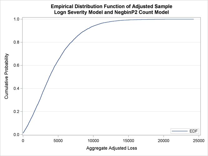
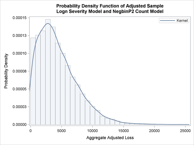
The empirical distribution function (EDF) and probability density function plots of the aggregate adjusted loss are shown in Output 18.1.4. Both plots indicate a heavy-tailed distribution of the total amount paid.
Output 18.1.4: PDF and EDF Plots of the Compound Distribution of the Total Amount Paid
|
|
|
Now consider that, in the future, you want to modify the policy provisions to add a limit on the total amount of payment that
is made to an individual policyholder in one year and to impose a group limit of 15,000 on the total amount of payments that
are made to the group as a whole in one year. You can analyze the effects of these modified policy provisions on the distribution
of the aggregate paid amount by recording the individual policyholder’s annual limit in the AnnualLimit variable of the input data set and then modifying your severity adjustment program by using the placeholder symbols _CUMADJSEVFOROBS_
and _CUMADJSEV_ as shown in the following PROC HPCDM step:
/* Simulate the aggregate loss distribution and aggregate adjusted
   loss distribution for the modified set of policy provisions */
proc hpcdm data=groupOfPolicies nreplicates=10000 seed=13579 print=all
           countstore=work.countregmodel severityest=work.sevregest
           plots=none nperturbedSamples=50
           adjustedseverity=amountPaid;
   severitymodel logn;

   if (_sev_ <= lowDeductible) then
      amountPaid = 0;
   else do;
      if (_sev_ <= highDeductible) then
         amountPaid = highDeductible *
            (_sev_-lowDeductible)/(highDeductible-lowDeductible);
      else
         amountPaid = MIN(_sev_, limit); /* imposes per-loss payment limit */

      /* impose policyholder's annual limit */
      amountPaid = MIN(amountPaid, MAX(0,annualLimit - _cumadjsevforobs_));

      /* impose group's annual limit */
      amountPaid = MIN(amountPaid, MAX(0,15000 - _cumadjsev_));
   end;
run;
The results of the perturbation analysis for these modified policy provisions are shown in Output 18.1.5. When compared to the results of Output 18.1.3, the additional policy provisions of restricting the total payment to the policyholder and the group have kept the median
payment unchanged, but the provisions have reduced the worst-case payment (99.5th percentile) to 14,683 440 from 15,588 1,197.
Output 18.1.5: Perturbation Summary of the Total Amount Paid for Modified Policy Provisions
| Adjusted Sample Percentile Perturbation Analysis |
||
|---|---|---|
| Percentile | Estimate | Standard Error |
| 0 | 0 | 0 |
| 1 | 7.96974 | 20.33033 |
| 5 | 398.70254 | 113.56342 |
| 25 | 1995.0 | 290.18465 |
| 50 | 3785.9 | 420.19002 |
| 75 | 6119.1 | 569.62667 |
| 95 | 10377.5 | 795.71616 |
| 99 | 13767.5 | 855.56936 |
| 99.5 | 14683.0 | 440.01020 |
| Number of Perturbed Samples = 50 | ||
| Size of Each Sample = 10000 | ||