The COPULA Procedure

Suppose the correlation structure required for a normal copula function is already given. For example, it can be estimated from the historic data on default times in some set of industries, but this stage is not in the scope of this example. The correlation structure is saved in a SAS data set called Inparm. The following statements and their output in Output 11.2.1 show that the correlation parameter is set at 0.8:

proc print data = inparm;
run;

Now you use PROC COPULA to simulate the data. The VAR statement specifies the list of variables to contain simulated data. The DEFINE statement assigns the name COP and specifies a normal copula that reads the correlation matrix from the inparm data set.

The SIMULATE statement refers to the COP label defined in the VAR statement and specifies some options: the NDRAWS= option specifies a sample size, the SEED= option specifies 1234 as the random number generator seed, the OUTUNIFORM=NORMAL_UNIFDATA option names the output data set for the result of simulation in uniforms, and the PLOTS= option requests the matrix of data scatter plots and marginal distributions (DATATYPE=ORIGINAL) and theoretical cumulative distribution function contour and surface plots (DISTRIBUTION=CDF). Theoretical distribution graphs work only for the bivariate case.

/* simulate the data from bivariate normal copula */
proc copula ;
   var Y1-Y2;
   define cop normal (corr=inparm);
   simulate cop /
            ndraws     = 500
            seed       = 1234
            outuniform = normal_unifdata
            plots      = (datatype = original
                          distribution = cdf);
run;

The graphical output is shown in Output 11.2.2 and in Output 11.2.3.

Output 11.2.2: Simulated Data, Uniform Marginals

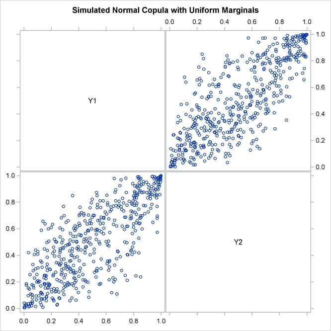
Output 11.2.2 shows bivariate scatter plots of the simulated data. Also note that due to the high correlation parameter (0.8), the scatter plots are most dense around the 45 degree line, which indicates high dependence between the two variables.

Output 11.2.3: Joint Cumulative Distribution

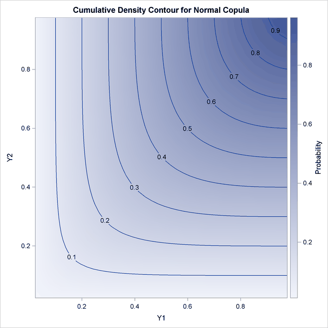
Output 11.2.3 shows the theoretical CDF contour plot. If the correlation parameter were set to 0, then knowing copula properties you would expect perfectly parallel straight lines with the slope of –45 degrees. On the other hand, if the parameter were set to 1, you would expect perpendicular lines with corners lying on the diagonal.

The next DATA step transforms the variables from zero-one uniformly distributed to nonnegative exponentially distributed with parameter 0.5. Three indicator variables are added to the data set as well. SURVIVE1 and SURVIVE2 are equal to 1 if a respective company has remained in business for more than three years. SURVIVE is equal to 1 if both companies survived the same period together.

/* default time has exponential marginal distribution with parameter 0.5 */
data default;
   set normal_unifdata;
   array arr{2} Y1-Y2;
   array time{2} time1-time2;
   array surv{2} survive1-survive2;
   lambda = 0.5;
   do i=1 to 2;
      time[i] = -log(1-arr[i])/lambda;
      surv[i] = 0;
      if (time[i] >3) then surv[i]=1;
   end;
   survive = 0;
   if (time1 >3) && (time2 >3) then survive = 1;
run;

The first analysis step is to look at correlations between survival times of two companies. This step is performed with the following CORR procedure:

proc corr data = default plot=matrix kendall;
   var time1 time2;
run;

The output of this code is given in Output 11.2.4 and in Output 11.2.5.

Output 11.2.4 shows some descriptive statistics and two measures of correlation: Pearson and Kendall. Both of these measures indicate high and statistically significant dependence between life spans of two companies.

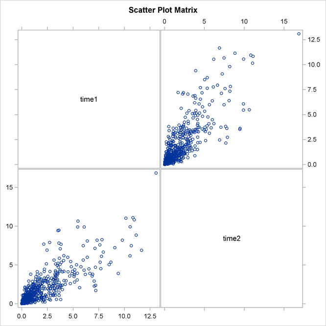
Output 11.2.5 shows marginal distributions and scatter plots of simulated data. Distributions are noticeably close to exponential and scatter plots show a high degree of dependence.

Output 11.2.5: Default Times

The second and the last step is to empirically estimate the default probabilities of two companies. This is done in the following FREQ procedure:

proc freq data=default;
   table survive survive1-survive2;
run;

The result is shown in Output 11.2.6.

Output 11.2.6 shows that the empirical default probabilities are 75% and 78%. Assuming that these companies are independent gives the probability estimate of both companies defaulting during the period of three years as: 0.75*0.78=0.59 (59%). Comparing this naive estimate with the much higher actual 83% joint default probability illustrates that neglecting the correlation between the two companies significantly underestimates the probability of default.