The COPULA Procedure

Hierarchical Archimedean Copula (HAC)

(Experimental)

Subsections:

Simulation

Adopting the notations of Savu and Trede (2010), let L denote the total level of hierarchies and let D denote the dimension of the HAC. There are $n_ l$ distinct copulas at each level $l,l=1,\ldots , L$ . These copulas are indexed by $(l,j),j=1,\ldots ,n_ l$ . At each level, there are also $d_ l$ variables, $0\leq d_ l\leq D$ and $\sum _ l d_ l =D$ . In the first step, all the variables at the lowest level are grouped into $n_1$ subsets, each subset being an ordinary multivariate Archimedean copula

$C_{1,j}(\bm {u}_{1,j})=\phi _{1,j}^{-1}\left(\sum _{\bm {u}_{1,j}} \phi _{1,j}(\bm {u}_{1,j})\right), j=1,\ldots ,n_1$

where $\phi _{1,j}$ is the generator of copula $C_{1,j}$ , $\bm {u}_{1,j}$ denotes the variables that belong to copula $C_{1,j}$ , and the sum $\sum _{u_{1,j}}$ is the sum over each variable in the subset $\bm {u}_{1,j}$ . The copulas $C_{1,j}$ can be different Archimedean copulas for $j=1,\ldots ,n_1$ . Then at the second level, the copulas $C_{1,j}$ that are derived in the first level are aggregated as if they are individual variables. Suppose there are $n_2$ copulas and $d_2$ variables,

$C_{2,j}(\bm {C}_{1,j},\bm {u}_{2,j}) =\phi _{2,j}^{-1}\left(\sum _{\bm {C}_{1,j}} \phi _{2,j}(\bm {C}_{1,j})+\sum _{\bm {u}_{2,j}} \phi _{2,j}(\bm {u}_{2,j})\right)$

where $\phi _{2,j}$ denotes the generator of $C_{2,j}$ and $\bm {C}_{1,j}$ represents the subset of copulas in $C_{1,h} ,h=1,\ldots ,n_1$ , that is aggregated for copula $C_{2,j}$ for $j=1,\ldots ,n_2$ . This structure continues until at level $l=L$ a single copula $C_{L,1}$ aggregates all the copulas at its previous level, $l=L-1$ .

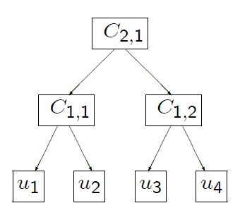
A four-dimensional example that has total levels $L=2$ and a structure shown in Figure 11.5 is defined as follows:

$\begin{align*} C_{2,1}(u_1,u_2,u_3,u_4) & = C_{2,1}\left(C_{1,1}(u_1, u_2),C_{1,2}(u_3, u_4)\right) \\ & =\phi ^{-1}_{2,1}\left(\phi _{2,1}\circ \phi ^{-1}_{1,1}\left(\phi _{1,1}(u_1)+\phi _{1,1}(u_2)\right)+\phi _{2,1}\circ \phi ^{-1}_{1,2} \left(\phi _{1,2}(u_3)+\phi _{1,2}(u_4)\right)\right) \end{align*}$

Figure 11.5: Example Four-Dimensional Hierarchical Structure with Two Levels

Theorem 4.4 of McNeil (2008) states that the sufficient condition for a general hierarchical Archimedean structure to be a proper copula is that all appearing nodes of the form $\phi _{m,j}\circ \phi ^{-1}_{n,j}$ have completely monotone derivatives. This condition places certain constraints on the copula parameters. In particular, if all the copulas in a hierarchical structure come from the Frank, Clayton, or Gumbel family, then $\theta _{m,j} \leq \theta _{n,j}$ for all j when $m<n$ . Intuitively, this means that rank correlation must be increasing as you move down the hierarchical structure.

The hierarchical Archimedean copulas available in the COPULA procedure are the hierarchical versions of the Clayton, Frank, and Gumbel copulas.

Simulation

A slightly modified version of the recursive algorithm from McNeil (2008) works for all valid hierarchical structures that have Clayton, Frank, or Gumbel generators:

Start at $l=L$ , and generate a random variable V with the distribution function F with Laplace transform $\phi _{L,1}^{-1}$ .
For $l=L-1,\ldots ,1$ , generate $u_{l,j}$ from its parent hierarchy. For $C_{l,j}$ , recursively call this algorithm with the proper inner generators that correspond to the copula family.
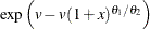
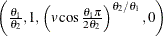
Return $\bm U= (\phi _{L,1}^{-1}(-\log (u_1)/V),\ldots , \phi _{L,1}^{-1}(-\log (u_ D)/V))^ T$ .

Let $\phi _1$ be the outer generator and $\phi _2$ the nested generator, and let $\theta _1$ and $\theta _2$ be the respective generator parameters. Let v be a draw from distribution function F with Laplace transform $\phi _1^{-1}$ . The inner copula generators $\phi _{12}(\cdot ;v)=\exp (-v\phi _1\circ \phi _2^{-1}(\cdot ))$ and their corresponding Laplace transform distributions for the Clayton, Frank, and Gumbel family are summarized in Table 11.3.

Table 11.3: Inner Generators and Corresponding Distributions

Copula Type	$\phi _{12}(x;v)$	Distribution with LT $\phi _{12}(\cdot ;v)$
Clayton	$\exp \left(v-v(1+x)^{\theta _1/\theta _2}\right)$	Tiled stable
Gumbel	$\exp (-vx^{\theta _1/\theta _2})$	Stable $\left(\frac{\theta _1}{\theta _2},1,\left(v\cos \frac{\theta _1\pi }{2\theta _2}\right)^{\theta _2/\theta _1},0\right)$
Frank	$\left(\frac{1}{1-e^{-\theta _1}}\left(1-\left(1-(1-e^{-\theta _2})\exp (-x)\right)^{\theta _1/\theta _2}\right)\right)^ v$	No closed form

Note that when $\theta _1=\theta _2$ , the inner generators for the Clayton and Gumbel family both simplify to the generator of the independence copula, $\exp (-vx)$ . For more information about simulating from the distribution with the Laplace transform given by the inner generator for the Frank family, see Hofert (2011). For more information about how to simulate from a tilted stable distribution, see McNeil (2008).