The X12 Procedure
- Overview
-
Getting Started

-
Syntax
Functional Summary PROC X12 Statement ADJUST Statement ARIMA Statement AUTOMDL Statement BY Statement CHECK Statement ESTIMATE Statement EVENT Statement FORECAST Statement ID Statement IDENTIFY Statement INPUT Statement OUTLIER Statement OUTPUT Statement REGRESSION Statement TABLES Statement TRANSFORM Statement USERDEFINED Statement VAR Statement X11 Statement
-
Details
-
Examples
- References
Example 37.5 Automatic Outlier Detection
This example demonstrates the use of the OUTLIER statement to automatically detect and remove outliers from a time series to be seasonally adjusted. The data set is the same as in the section Basic Seasonal Adjustment and the previous examples. Adding the OUTLIER statement to Example 37.3 requests that outliers be detected by using the default critical value as described in the section OUTLIER Statement. The tables associated with outlier detection for this example are shown in Output 37.5.1. The first table shows the critical values; the second table shows that a single potential outlier was identified; the third table shows the estimates for the ARMA parameters. Since no outliers are included in the regression model, the "Regression Model Parameter Estimates" table is not displayed. Because only a potential outlier was identified, and not an actual outlier, in this case the A1 series and the B1 series are identical.
title 'Automatic Outlier Identification';
proc x12 data=sales date=date;
   var sales;
   transform function=log;
   arima model=( (0,1,1)(0,1,1) );
   outlier;
   estimate;
   x11;
   output out=nooutlier a1 b1 d10;
run ;
| Automatic Outlier Identification |
| Critical Values to use in Outlier Detection |
|
|---|---|
| For Variable sales | |
| Begin | SEP1978 |
| End | AUG1990 |
| Observations | 144 |
| Method | Add One |
| AO Critical Value | 3.889838 |
| LS Critical Value | 3.889838 |
| Note: | The following time series values might later be identified as outliers when data are added or revised. They were not identified as outliers in this run either because their test t-statistics were slightly below the critical value or because they were eliminated during the backward deletion step of the identification procedure, when a non-robust t-statistic is used. |
| Potential Outliers | |||
|---|---|---|---|
| For Variable sales | |||
| Type of Outlier | Date | t Value for AO | t Value for LS |
| AO | NOV1989 | -3.48 | -1.51 |
| Exact ARMA Maximum Likelihood Estimation | |||||
|---|---|---|---|---|---|
| For Variable sales | |||||
| Parameter | Lag | Estimate | Standard Error | t Value | Pr > |t| |
| Nonseasonal MA | 1 | 0.40181 | 0.07887 | 5.09 | <.0001 |
| Seasonal MA | 12 | 0.55695 | 0.07626 | 7.30 | <.0001 |
In the next example, reducing the critical value to 3.3 causes the outlier identification routine to more aggressively identify outliers as shown in Output 37.5.2. The first table shows the critical values. The second table shows that three additive outliers and a level shift have been included in the regression model. The third table shows how the inclusion of outliers in the model affects the ARMA parameters.
proc x12 data=sales date=date;
   var sales;
   transform function=log;
   arima model=((0,1,1) (0,1,1));
   outlier cv=3.3;
   estimate;
   x11;
   output out=outlier(obs=50) a1 a8  a8ao a8ls b1 d10;
run;
proc print data=outlier(obs=50);
run;
| Automatic Outlier Identification |
| Critical Values to use in Outlier Detection |
|
|---|---|
| For Variable sales | |
| Begin | SEP1978 |
| End | AUG1990 |
| Observations | 144 |
| Method | Add One |
| AO Critical Value | 3.3 |
| LS Critical Value | 3.3 |
| Regression Model Parameter Estimates | ||||||
|---|---|---|---|---|---|---|
| For Variable sales | ||||||
| Type | Parameter | NoEst | Estimate | Standard Error | t Value | Pr > |t| |
| Automatically Identified | AO JAN1981 | Est | 0.09590 | 0.02168 | 4.42 | <.0001 |
| LS FEB1983 | Est | -0.09673 | 0.02488 | -3.89 | 0.0002 | |
| AO OCT1983 | Est | -0.08032 | 0.02146 | -3.74 | 0.0003 | |
| AO NOV1989 | Est | -0.10323 | 0.02480 | -4.16 | <.0001 | |
| Exact ARMA Maximum Likelihood Estimation | |||||
|---|---|---|---|---|---|
| For Variable sales | |||||
| Parameter | Lag | Estimate | Standard Error | t Value | Pr > |t| |
| Nonseasonal MA | 1 | 0.33205 | 0.08239 | 4.03 | <.0001 |
| Seasonal MA | 12 | 0.49647 | 0.07676 | 6.47 | <.0001 |
The first 50 observations of the A1, A8, A8AO, A8LS, B1, and D10 series are displayed in Output 37.5.3. You can confirm the following relationships from the data:
 |
 |
The seasonal factors are stored in the variable sales_D10.
| Automatic Outlier Identification |
| Obs | DATE | sales_A1 | sales_A8 | sales_A8AO | sales_A8LS | sales_B1 | sales_D10 |
|---|---|---|---|---|---|---|---|
| 1 | SEP78 | 112 | 1.10156 | 1.00000 | 1.10156 | 101.674 | 0.90496 |
| 2 | OCT78 | 118 | 1.10156 | 1.00000 | 1.10156 | 107.121 | 0.94487 |
| 3 | NOV78 | 132 | 1.10156 | 1.00000 | 1.10156 | 119.830 | 1.04711 |
| 4 | DEC78 | 129 | 1.10156 | 1.00000 | 1.10156 | 117.107 | 1.00119 |
| 5 | JAN79 | 121 | 1.10156 | 1.00000 | 1.10156 | 109.844 | 0.94833 |
| 6 | FEB79 | 135 | 1.10156 | 1.00000 | 1.10156 | 122.553 | 1.06817 |
| 7 | MAR79 | 148 | 1.10156 | 1.00000 | 1.10156 | 134.355 | 1.18679 |
| 8 | APR79 | 148 | 1.10156 | 1.00000 | 1.10156 | 134.355 | 1.17607 |
| 9 | MAY79 | 136 | 1.10156 | 1.00000 | 1.10156 | 123.461 | 1.07565 |
| 10 | JUN79 | 119 | 1.10156 | 1.00000 | 1.10156 | 108.029 | 0.91844 |
| 11 | JUL79 | 104 | 1.10156 | 1.00000 | 1.10156 | 94.412 | 0.81206 |
| 12 | AUG79 | 118 | 1.10156 | 1.00000 | 1.10156 | 107.121 | 0.91602 |
| 13 | SEP79 | 115 | 1.10156 | 1.00000 | 1.10156 | 104.397 | 0.90865 |
| 14 | OCT79 | 126 | 1.10156 | 1.00000 | 1.10156 | 114.383 | 0.94131 |
| 15 | NOV79 | 141 | 1.10156 | 1.00000 | 1.10156 | 128.000 | 1.04496 |
| 16 | DEC79 | 135 | 1.10156 | 1.00000 | 1.10156 | 122.553 | 0.99766 |
| 17 | JAN80 | 125 | 1.10156 | 1.00000 | 1.10156 | 113.475 | 0.94942 |
| 18 | FEB80 | 149 | 1.10156 | 1.00000 | 1.10156 | 135.263 | 1.07172 |
| 19 | MAR80 | 170 | 1.10156 | 1.00000 | 1.10156 | 154.327 | 1.18663 |
| 20 | APR80 | 170 | 1.10156 | 1.00000 | 1.10156 | 154.327 | 1.18105 |
| 21 | MAY80 | 158 | 1.10156 | 1.00000 | 1.10156 | 143.433 | 1.07383 |
| 22 | JUN80 | 133 | 1.10156 | 1.00000 | 1.10156 | 120.738 | 0.91930 |
| 23 | JUL80 | 114 | 1.10156 | 1.00000 | 1.10156 | 103.490 | 0.81385 |
| 24 | AUG80 | 140 | 1.10156 | 1.00000 | 1.10156 | 127.093 | 0.91466 |
| 25 | SEP80 | 145 | 1.10156 | 1.00000 | 1.10156 | 131.632 | 0.91302 |
| 26 | OCT80 | 150 | 1.10156 | 1.00000 | 1.10156 | 136.171 | 0.93086 |
| 27 | NOV80 | 178 | 1.10156 | 1.00000 | 1.10156 | 161.589 | 1.03965 |
| 28 | DEC80 | 163 | 1.10156 | 1.00000 | 1.10156 | 147.972 | 0.99440 |
| 29 | JAN81 | 172 | 1.21243 | 1.10065 | 1.10156 | 141.864 | 0.95136 |
| 30 | FEB81 | 178 | 1.10156 | 1.00000 | 1.10156 | 161.589 | 1.07981 |
| 31 | MAR81 | 199 | 1.10156 | 1.00000 | 1.10156 | 180.653 | 1.18661 |
| 32 | APR81 | 199 | 1.10156 | 1.00000 | 1.10156 | 180.653 | 1.19097 |
| 33 | MAY81 | 184 | 1.10156 | 1.00000 | 1.10156 | 167.036 | 1.06905 |
| 34 | JUN81 | 162 | 1.10156 | 1.00000 | 1.10156 | 147.064 | 0.92446 |
| 35 | JUL81 | 146 | 1.10156 | 1.00000 | 1.10156 | 132.539 | 0.81517 |
| 36 | AUG81 | 166 | 1.10156 | 1.00000 | 1.10156 | 150.695 | 0.91148 |
| 37 | SEP81 | 171 | 1.10156 | 1.00000 | 1.10156 | 155.234 | 0.91352 |
| 38 | OCT81 | 180 | 1.10156 | 1.00000 | 1.10156 | 163.405 | 0.91632 |
| 39 | NOV81 | 193 | 1.10156 | 1.00000 | 1.10156 | 175.206 | 1.03194 |
| 40 | DEC81 | 181 | 1.10156 | 1.00000 | 1.10156 | 164.312 | 0.98879 |
| 41 | JAN82 | 183 | 1.10156 | 1.00000 | 1.10156 | 166.128 | 0.95699 |
| 42 | FEB82 | 218 | 1.10156 | 1.00000 | 1.10156 | 197.901 | 1.09125 |
| 43 | MAR82 | 230 | 1.10156 | 1.00000 | 1.10156 | 208.795 | 1.19059 |
| 44 | APR82 | 242 | 1.10156 | 1.00000 | 1.10156 | 219.688 | 1.20448 |
| 45 | MAY82 | 209 | 1.10156 | 1.00000 | 1.10156 | 189.731 | 1.06355 |
| 46 | JUN82 | 191 | 1.10156 | 1.00000 | 1.10156 | 173.391 | 0.92897 |
| 47 | JUL82 | 172 | 1.10156 | 1.00000 | 1.10156 | 156.142 | 0.81476 |
| 48 | AUG82 | 194 | 1.10156 | 1.00000 | 1.10156 | 176.114 | 0.90667 |
| 49 | SEP82 | 196 | 1.10156 | 1.00000 | 1.10156 | 177.930 | 0.91200 |
| 50 | OCT82 | 196 | 1.10156 | 1.00000 | 1.10156 | 177.930 | 0.89970 |
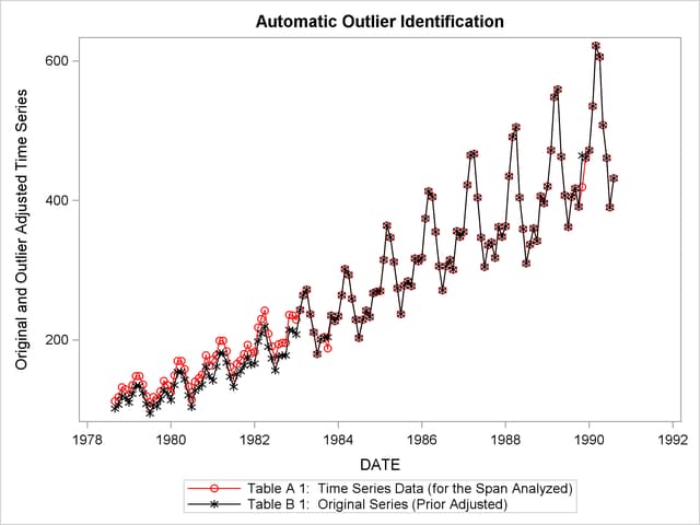
From the two previous examples, you can examine how outlier detection affects the seasonally adjusted series. Output 37.5.4 shows a plot of A1 versus B1 in the series where outliers are detected. B1 has been adjusted for the additive outliers and the level shift.
proc sgplot data=outlier;
   series x=date y=sales_A1 / name='A1' markers
                              markerattrs=(color=red symbol='circle')
                              lineattrs=(color=red);
   series x=date y=sales_B1 / name='B1' markers
                              markerattrs=(color=black symbol='asterisk')
                              lineattrs=(color=black);
   yaxis label='Original and Outlier Adjusted Time Series';
run;
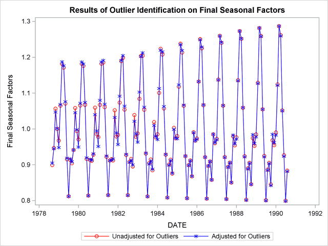
Output 37.5.5 compares the seasonal factors (table D10) of the series unadjusted for outliers to the series adjusted for outliers. The seasonal factors are based on the B1 series.
data both;
   merge nooutlier(rename=(sales_D10=unadj_D10)) outlier;
run;

title 'Results of Outlier Identification on Final Seasonal Factors';
proc sgplot data=both;
   series x=date y=unadj_D10 / name='unadjusted' markers
                               markerattrs=(color=red symbol='circle')
                               lineattrs=(color=red)
                               legendlabel='Unadjusted for Outliers';
   series x=date y=sales_D10 / name='adjusted' markers
                               markerattrs=(color=blue symbol='asterisk')
                               lineattrs=(color=blue)
                               legendlabel='Adjusted for Outliers';
   yaxis label='Final Seasonal Factors';
run;