The X12 Procedure
- Overview
-
Getting Started

-
Syntax
Functional Summary PROC X12 Statement ADJUST Statement ARIMA Statement AUTOMDL Statement BY Statement CHECK Statement ESTIMATE Statement EVENT Statement FORECAST Statement ID Statement IDENTIFY Statement INPUT Statement OUTLIER Statement OUTPUT Statement REGRESSION Statement TABLES Statement TRANSFORM Statement USERDEFINED Statement VAR Statement X11 Statement
-
Details
-
Examples
- References
Example 37.1 ARIMA Model Identification
This example shows typical PROC X12 statements that are used for ARIMA model identification. This example invokes the X12 procedure and uses the TRANSFORM and IDENTIFY statements. It specifies the time series data, takes the logarithm of the series (TRANSFORM statement), and generates ACFs and PACFs for the specified levels of differencing (IDENTIFY statement). The ACFs and PACFs for DIFF=1 and SDIFF=1 are shown in Output 37.1.1, Output 37.1.2, Output 37.1.3, and Output 37.1.4. The data set is the same as in the section Basic Seasonal Adjustment.
The graphical displays are available when ODS Graphics is enabled. For more information about the graphics available in the X12 procedure, see the section ODS Graphics.
proc x12 data=sales date=date;
   var sales;
   transform power=0;
   identify diff=(0,1) sdiff=(0,1);
run;
Output 37.1.1
ACFs (Nonseasonal Order=1 Seasonal Order=1)
The X12 Procedure
| Autocorrelation of Regression Residuals for ARIMA Model Identification | |||||
|---|---|---|---|---|---|
| For Variable sales | |||||
| Differencing: Nonseasonal Order=1 Seasonal Order=1 | |||||
| Lag | Correlation | Standard Error | Chi-Square | DF | Pr > ChiSq |
| 1 | -0.34112 | 0.08737 | 15.5957 | 1 | <.0001 |
| 2 | 0.10505 | 0.09701 | 17.0860 | 2 | 0.0002 |
| 3 | -0.20214 | 0.09787 | 22.6478 | 3 | <.0001 |
| 4 | 0.02136 | 0.10101 | 22.7104 | 4 | 0.0001 |
| 5 | 0.05565 | 0.10104 | 23.1387 | 5 | 0.0003 |
| 6 | 0.03080 | 0.10128 | 23.2709 | 6 | 0.0007 |
| 7 | -0.05558 | 0.10135 | 23.7050 | 7 | 0.0013 |
| 8 | -0.00076 | 0.10158 | 23.7050 | 8 | 0.0026 |
| 9 | 0.17637 | 0.10158 | 28.1473 | 9 | 0.0009 |
| 10 | -0.07636 | 0.10389 | 28.9869 | 10 | 0.0013 |
| 11 | 0.06438 | 0.10432 | 29.5887 | 11 | 0.0018 |
| 12 | -0.38661 | 0.10462 | 51.4728 | 12 | <.0001 |
| 13 | 0.15160 | 0.11501 | 54.8664 | 13 | <.0001 |
| 14 | -0.05761 | 0.11653 | 55.3605 | 14 | <.0001 |
| 15 | 0.14957 | 0.11674 | 58.7204 | 15 | <.0001 |
| 16 | -0.13894 | 0.11820 | 61.6452 | 16 | <.0001 |
| 17 | 0.07048 | 0.11944 | 62.4045 | 17 | <.0001 |
| 18 | 0.01563 | 0.11975 | 62.4421 | 18 | <.0001 |
| 19 | -0.01061 | 0.11977 | 62.4596 | 19 | <.0001 |
| 20 | -0.11673 | 0.11978 | 64.5984 | 20 | <.0001 |
| 21 | 0.03855 | 0.12064 | 64.8338 | 21 | <.0001 |
| 22 | -0.09136 | 0.12074 | 66.1681 | 22 | <.0001 |
| 23 | 0.22327 | 0.12126 | 74.2099 | 23 | <.0001 |
| 24 | -0.01842 | 0.12436 | 74.2652 | 24 | <.0001 |
| 25 | -0.10029 | 0.12438 | 75.9183 | 25 | <.0001 |
| 26 | 0.04857 | 0.12500 | 76.3097 | 26 | <.0001 |
| 27 | -0.03024 | 0.12514 | 76.4629 | 27 | <.0001 |
| 28 | 0.04713 | 0.12520 | 76.8387 | 28 | <.0001 |
| 29 | -0.01803 | 0.12533 | 76.8943 | 29 | <.0001 |
| 30 | -0.05107 | 0.12535 | 77.3442 | 30 | <.0001 |
| 31 | -0.05377 | 0.12551 | 77.8478 | 31 | <.0001 |
| 32 | 0.19573 | 0.12569 | 84.5900 | 32 | <.0001 |
| 33 | -0.12242 | 0.12799 | 87.2543 | 33 | <.0001 |
| 34 | 0.07775 | 0.12888 | 88.3401 | 34 | <.0001 |
| 35 | -0.15245 | 0.12924 | 92.5584 | 35 | <.0001 |
| 36 | -0.01000 | 0.13061 | 92.5767 | 36 | <.0001 |
| Note: | The P-values approximate the probability of observing a Chi-Square at least this large when the model fitted is correct. When DF is positive, small values of P, customarily those below 0.05, indicate model inadequacy. |
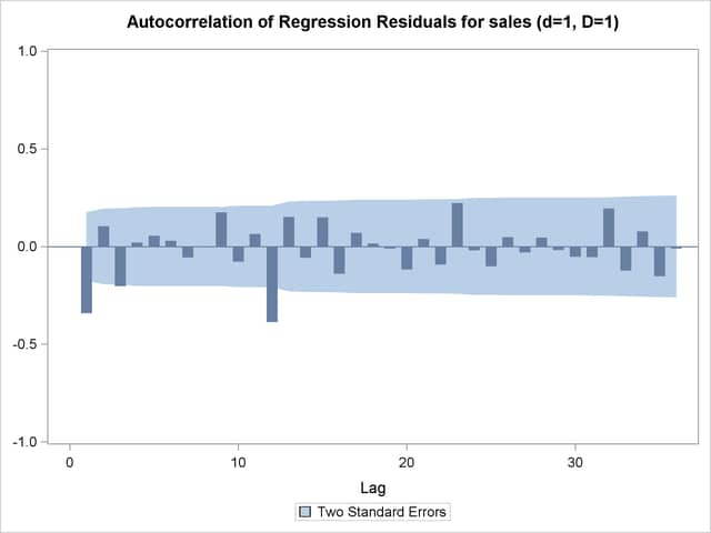
Output 37.1.2
Plot for ACFs (Nonseasonal Order=1 Seasonal Order=1)
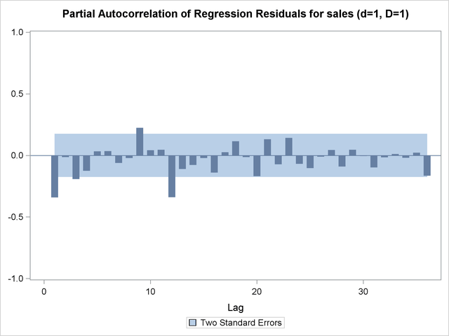
Output 37.1.3
PACFs (Nonseasonal Order=1 Seasonal Order=1)
| Partial Autocorrelations of Regression Residuals for ARIMA Model Identification |
||
|---|---|---|
| For Variable sales | ||
| Differencing: Nonseasonal Order=1 Seasonal Order=1 |
||
| Lag | Correlation | Standard Error |
| 1 | -0.34112 | 0.08737 |
| 2 | -0.01281 | 0.08737 |
| 3 | -0.19266 | 0.08737 |
| 4 | -0.12503 | 0.08737 |
| 5 | 0.03309 | 0.08737 |
| 6 | 0.03468 | 0.08737 |
| 7 | -0.06019 | 0.08737 |
| 8 | -0.02022 | 0.08737 |
| 9 | 0.22558 | 0.08737 |
| 10 | 0.04307 | 0.08737 |
| 11 | 0.04659 | 0.08737 |
| 12 | -0.33869 | 0.08737 |
| 13 | -0.10918 | 0.08737 |
| 14 | -0.07684 | 0.08737 |
| 15 | -0.02175 | 0.08737 |
| 16 | -0.13955 | 0.08737 |
| 17 | 0.02589 | 0.08737 |
| 18 | 0.11482 | 0.08737 |
| 19 | -0.01316 | 0.08737 |
| 20 | -0.16743 | 0.08737 |
| 21 | 0.13240 | 0.08737 |
| 22 | -0.07204 | 0.08737 |
| 23 | 0.14285 | 0.08737 |
| 24 | -0.06733 | 0.08737 |
| 25 | -0.10267 | 0.08737 |
| 26 | -0.01007 | 0.08737 |
| 27 | 0.04378 | 0.08737 |
| 28 | -0.08995 | 0.08737 |
| 29 | 0.04690 | 0.08737 |
| 30 | -0.00490 | 0.08737 |
| 31 | -0.09638 | 0.08737 |
| 32 | -0.01528 | 0.08737 |
| 33 | 0.01150 | 0.08737 |
| 34 | -0.01916 | 0.08737 |
| 35 | 0.02303 | 0.08737 |
| 36 | -0.16488 | 0.08737 |
Output 37.1.4
Plot for PACFs (Nonseasonal Order=1 Seasonal Order=1)