The VARMAX Procedure
- Overview
-
Getting Started

-
Syntax
-
Details
Missing Values VARMAX Model Dynamic Simultaneous Equations Modeling Impulse Response Function Forecasting Tentative Order Selection VAR and VARX Modeling Bayesian VAR and VARX Modeling VARMA and VARMAX Modeling Model Diagnostic Checks Cointegration Vector Error Correction Modeling I(2) Model Multivariate GARCH Modeling Output Data Sets OUT= Data Set OUTEST= Data Set OUTHT= Data Set OUTSTAT= Data Set Printed Output ODS Table Names ODS Graphics Computational Issues
-
Examples
- References
| Forecasting |
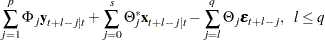
The optimal (minimum MSE)  -step-ahead forecast of
  is
is
 |
 |
 |
|||
 |
|
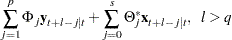 |
with  and
and  for
for  . For the forecasts
  , see the section State-Space Representation.
Covariance Matrices of Prediction Errors without Exogenous (Independent) Variables
Under the stationarity assumption, the optimal (minimum MSE) -step-ahead forecast of has an infinite moving-average form, 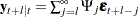 . The prediction error of the optimal -step-ahead forecast is
  , with zero mean and covariance matrix,
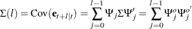 |
where  with a lower triangular matrix
  such that
  . Under the assumption of normality of the
  , the -step-ahead prediction error
  is also normally distributed as multivariate
  . Hence, it follows that the diagonal elements
  of
of  can be used, together with the point forecasts
  , to construct -step-ahead prediction intervals of the future values of the component series,
  .
.
The following statements use the COVPE option to compute the covariance matrices of the prediction errors for a VAR(1) model. The parts of the VARMAX procedure output are shown in Figure 35.36 and Figure 35.37.
proc varmax data=simul1;
   model y1 y2 / p=1 noint lagmax=5
                 printform=both
                 print=(decompose(5) impulse=(all) covpe(5));
run;
Figure 35.36 is the output in a matrix format associated with the COVPE option for the prediction error covariance matrices.
| Prediction Error Covariances | |||
|---|---|---|---|
| Lead | Variable | y1 | y2 |
| 1 | y1 | 1.28875 | 0.39751 |
| y2 | 0.39751 | 1.41839 | |
| 2 | y1 | 2.92119 | 1.00189 |
| y2 | 1.00189 | 2.18051 | |
| 3 | y1 | 4.59984 | 1.98771 |
| y2 | 1.98771 | 3.03498 | |
| 4 | y1 | 5.91299 | 3.04856 |
| y2 | 3.04856 | 4.07738 | |
| 5 | y1 | 6.69463 | 3.85346 |
| y2 | 3.85346 | 5.07010 | |
Figure 35.37 is the output in a univariate format associated with the COVPE option for the prediction error covariances. This printing format more easily explains the prediction error covariances of each variable.
| Prediction Error Covariances by Variable | |||
|---|---|---|---|
| Variable | Lead | y1 | y2 |
| y1 | 1 | 1.28875 | 0.39751 |
| 2 | 2.92119 | 1.00189 | |
| 3 | 4.59984 | 1.98771 | |
| 4 | 5.91299 | 3.04856 | |
| 5 | 6.69463 | 3.85346 | |
| y2 | 1 | 0.39751 | 1.41839 |
| 2 | 1.00189 | 2.18051 | |
| 3 | 1.98771 | 3.03498 | |
| 4 | 3.04856 | 4.07738 | |
| 5 | 3.85346 | 5.07010 | |
Covariance Matrices of Prediction Errors in the Presence of Exogenous (Independent) Variables
Exogenous variables can be both stochastic and nonstochastic (deterministic) variables. Considering the forecasts in the VARMAX( ,
, ,
, ) model, there are two cases.
As defined in the section State-Space Representation,  has the representation
 |
and hence
 |
Therefore, the covariance matrix of the -step-ahead prediction error is given as
 |
where  is the covariance of the white noise series
  , and is the white noise series for the VARMA(,) model of exogenous (independent) variables, which is assumed not to be correlated with
  or its lags.
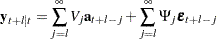
The optimal forecast of  conditioned on the past information and also on known future values
  can be represented as
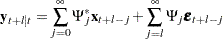 |
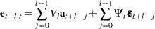
and the forecast error is
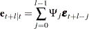 |
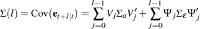
Thus, the covariance matrix of the -step-ahead prediction error is given as
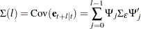 |
Decomposition of Prediction Error Covariances
In the relation 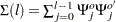 , the diagonal elements can be interpreted as providing a decomposition of the -step-ahead prediction error covariance
  for each component series
  into contributions from the components of the standardized innovations .
If you denote the ( )th element of
  by
by  , the MSE of
  is
is
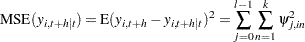 |
Note that  is interpreted as the contribution of innovations in variable
  to the prediction error covariance of the -step-ahead forecast of variable
  .
.
The proportion,  , of the -step-ahead forecast error covariance of variable accounting for the innovations in variable is
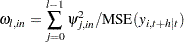 |
The following statements use the DECOMPOSE option to compute the decomposition of prediction error covariances and their proportions for a VAR(1) model:
proc varmax data=simul1;
   model y1 y2 / p=1 noint print=(decompose(15))
                 printform=univariate;
run;
The proportions of decomposition of prediction error covariances of two variables are given in Figure 35.38. The output explains that about 91.356% of the one-step-ahead prediction error covariances of the variable  is accounted for by its own innovations and about 8.644% is accounted for by
  innovations.
| Proportions of Prediction Error Covariances by Variable |
|||
|---|---|---|---|
| Variable | Lead | y1 | y2 |
| y1 | 1 | 1.00000 | 0.00000 |
| 2 | 0.88436 | 0.11564 | |
| 3 | 0.75132 | 0.24868 | |
| 4 | 0.64897 | 0.35103 | |
| 5 | 0.58460 | 0.41540 | |
| y2 | 1 | 0.08644 | 0.91356 |
| 2 | 0.31767 | 0.68233 | |
| 3 | 0.50247 | 0.49753 | |
| 4 | 0.55607 | 0.44393 | |
| 5 | 0.53549 | 0.46451 | |
Forecasting of the Centered Series
If the CENTER option is specified, the sample mean vector is added to the forecast.
Forecasting of the Differenced Series
If dependent (endogenous) variables are differenced, the final forecasts and their prediction error covariances are produced by integrating those of the differenced series. However, if the PRIOR option is specified, the forecasts and their prediction error variances of the differenced series are produced.
Let  be the original series with some appended zero values that correspond to the unobserved past observations. Let
  be the
  matrix polynomial in the backshift operator that corresponds to the differencing specified by the MODEL statement. The off-diagonal elements of
  are zero, and the diagonal elements can be different. Then
  .
.
This gives the relationship
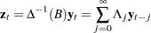 |
where 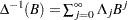 and
and  .
.
The -step-ahead prediction of  is
is
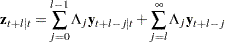 |
The -step-ahead prediction error of is
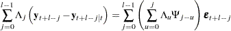 |
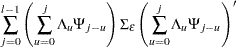
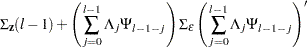
Letting  , the covariance matrix of the l-step-ahead prediction error of ,
  , is
, is
 |
|
 |
|||
 |
|
 |
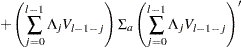
If there are stochastic exogenous (independent) variables, the covariance matrix of the l-step-ahead prediction error of , , is
|
|
 |
|||
|
|
 |