The SSM Procedure (Experimental)

Predefined Trend Models

The statistical models that govern the predefined trend components available in the SSM procedure are divided into two groups: models that are applicable to equally spaced data (possibly with replication), and the models that are applicable more generally (the irregular data type). Each trend component can be described as a dot product $\text{[math]}$ for some (time-invariant) vector $\text{[math]}$ and a state vector $\text{[math]}$ . The component specification is complete after the vector $\text{[math]}$ is specified and the system matrices that govern the equations of $\text{[math]}$ are specified. For trend models for regular data, all the system matrices are time-invariant. For irregular data, $\text{[math]}$ and $\text{[math]}$ depend on the spacing between the distinct time points: $\text{[math]}$ .

Trend Models for Regular Data

These models are applicable when the data type is either regular or regular-with-replication. A good reference for these models is Harvey (1989).

Random Walk Trend

This model provides a trend pattern in which the level of the curve changes slowly. The rapidity of this change is inversely proportional to the disturbance variance $\text{[math]}$ that governs the underlying state. It can be described as $\text{[math]}$ , where $\text{[math]}$ and the (one-dimensional) state $\text{[math]}$ follows a random walk:

$\text{[math]}$

Here $\text{[math]}$ and $\text{[math]}$ . The initial condition is fully diffuse.

Local Linear Trend

This model provides a trend pattern in which both the level and the slope of the curve vary slowly. This variation in the level and the slope is controlled by two parameters: $\text{[math]}$ controls the level variation, and $\text{[math]}$ controls the slope variation. If $\text{[math]}$ , the resulting trend is called an integrated random walk. Here $\text{[math]}$ , $\text{[math]}$ , and $\text{[math]}$ . 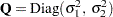The initial condition is fully diffuse.

Damped Local Linear Trend

This trend pattern is similar to the local linear trend pattern. However, in the DLL trend the slope follows a first-order autoregressive model whereas in the LL trend the slope follows a random walk. The autoregressive parameter or the damping factor, $\text{[math]}$ , must lie between 0.0 and 1.0, which implies that the long-run forecast according to this pattern has a slope that tends to zero. Here $\text{[math]}$ , $\text{[math]}$ , and $\text{[math]}$ . The initial condition is partially diffuse with $\text{[math]}$ .

Trend Models for Irregular Data

A good reference for these models is de Jong and Mazzi (2001). Throughout this section $\text{[math]}$ denotes the difference between the successive time points. The system matrices $\text{[math]}$ and $\text{[math]}$ that govern these models depend on $\text{[math]}$ . However, whenever the notation is unambiguous, the subscript $\text{[math]}$ is omitted.

Polynomial Spline Trend

This model is a general-purpose tool for extracting a smooth trend from the noisy data. The order of the spline governs the order of the local polynomial that defines the spline. In the SSM procedure the order is restricted to be an integer 1, 2, or 3; the default order is 1. The order 1 spline corresponds to a random walk, the order 2 spline corresponds to an integrated random walk, and the order 3 spline provides a locally quadratic trend. The dimension of the state underlying this component is the same as the order of the spline. The system matrices for the different orders are described below (in all the cases the initial condition is fully diffuse):

order=1: $\text{[math]}$ , $\text{[math]}$ , and $\text{[math]}$
order=2: $\text{[math]}$ , $\text{[math]}$ , and $\text{[math]}$
order=3: $\text{[math]}$ , $\text{[math]}$ , and

$\text{[math]}$

Decay and Growth Trends

There are two choices for the decay trend: DECAY and DECAY(OU). Similarly, there are two choices for the growth trend: GROWTH and GROWTH(OU). The "OU" stands for the Ornstein-Uhlenbeck form of these models. The decay trend is a sum of two correlated components: one component is a random walk, and the other component is a stationary autoregression. In its Ornstein-Uhlenbeck form, the random walk component is replaced by a constant. The growth trend (and its Ornstein-Uhlenbeck variant) has the same form as the decay trend except that the autorgression is nonstationary (in fact, it is explosive). Note that, in the case of the growth trend models, floating-point errors can result for even moderately long forecast horizons because of the explosive growth in the trend values.

The system matrices for the decay and the growth types in their respective cases are identical, except for the sign of the rate parameter $\text{[math]}$ : $\text{[math]}$ for the decay type, and $\text{[math]}$ for the growth type. In addition, the initial conditions for the growth models are fully diffuse; they are only partially diffuse for the decay models. The underlying state vector for all these models is two-dimensional.

The system matrices for the DECAY type are:

$\text{[math]}$	$\text{[math]}$	$\text{[math]}$
$\text{[math]}$	$\text{[math]}$	$\text{[math]}$
$\text{[math]}$	$\text{[math]}$	$\text{[math]}$

The initial condition is partially diffuse with 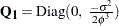$\text{[math]}$ . The system matrices for the GROWTH type are the same (with $\text{[math]}$ ), except that the initial condition is fully diffuse; so $\text{[math]}$ .

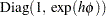
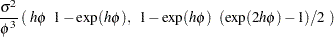
For the DECAY(OU) type, $\text{[math]}$ and $\text{[math]}$ are the same as DECAY, whereas

$\text{[math]}$

The system matrices for the GROWTH(OU) type are the same (with $\text{[math]}$ ), except that the initial condition is fully diffuse; so $\text{[math]}$ .

Note: This procedure is experimental.