The SSM Procedure (Experimental)

Likelihood, Filtering, and Smoothing

The Kalman filter and smoother (KFS) algorithm is the main computational tool for using SSM for data analysis. This subsection briefly describes the basic quantities generated by this algorithm and their relationship to the output generated by the SSM procedure. For proper treatment of SSMs with a diffuse initial condition or when regression variables are present, a modified version of the traditional KFS, called diffuse Kalman filter and smoother (DKFS), is needed. A good discussion of the different variants of the traditional and diffuse KFS can be found in Durbin and Koopman (2001). The DKFS implemented in the SSM procedure closely follows the treatment in de Jong and Chu-Chun-Lin (2003). Additional details can be found in these references.

The state space model equations (see the section The State Space Model and Notation) imply that the combined response data vector $\text{[math]}$ has a Gaussian probability distribution. This probability distribution is proper if $\text{[math]}$ , the dimension of the diffuse vector $\text{[math]}$ in the initial condition, is zero and if $\text{[math]}$ , the number of regression variables in the observation equation, is also zero (the regression parameter $\text{[math]}$ is also treated as a diffuse vector). Otherwise, this probability distribution is improper. The KFS algorithm is a combination of two iterative phases: a forward pass through the data, called filtering, and a backward pass through the data, called smoothing, that uses the quantities generated during filtering. One of the advantages of using the SSM formulation to analyze the time series data is its ability to handle the missing values in the response variables. The KFS algorithm appropriately handles the missing values in $\text{[math]}$ . For additional information about how PROC SSM handles missing values, see the section Missing Values.

Filtering Pass

The filtering pass sequentially computes the following quantities for $\text{[math]}$ and $\text{[math]}$ :

Table 27.5 KFS: Filtering Phase
$\text{[math]}$	One-step-ahead prediction of the response values
$\text{[math]}$	One-step-ahead prediction residuals
$\text{[math]}$	Variance of the one-step-ahead prediction
$\text{[math]}$	One-step-ahead prediction of the state vector
$\text{[math]}$	Covariance of $\text{[math]}$
$\text{[math]}$	$\text{[math]}$ -dimensional vector
$\text{[math]}$	$\text{[math]}$ -dimensional symmetric matrix
$\text{[math]}$	Estimate of $\text{[math]}$ and $\text{[math]}$ using the data up to $\text{[math]}$
$\text{[math]}$	Covariance of $\text{[math]}$

Here the notation $\text{[math]}$ denotes the conditional expectation of $\text{[math]}$ given the history up to the index $\text{[math]}$ : $\text{[math]}$ . Similarly $\text{[math]}$ denotes the corresponding conditional variance. $\text{[math]}$ is set to missing whenever $\text{[math]}$ is missing. In the diffuse case, the conditional expectations must be appropriately interpreted. The vector $\text{[math]}$ and the matrix $\text{[math]}$ contain some accumulated quantities that are needed for the estimation of $\text{[math]}$ and $\text{[math]}$ . Of course, when $\text{[math]}$ (the nondiffuse case), these quantities are not needed. In the diffuse case, as the matrix $\text{[math]}$ is sequentially accumulated (starting at $\text{[math]}$ ), it might not be invertible until some $\text{[math]}$ . The filtering process is called initialized after $\text{[math]}$ . In some situations, this initialization might not happen even after the entire sample is processed—that is, the filtering process remains uninitialized. This can happen if the regression variables are collinear or if the data are not sufficient to estimate the initial condition $\text{[math]}$ for some other reason.

The filtering process is used for a variety of purposes. One important use of filtering is to compute the likelihood of the data. In the model fitting phase, the unknown model parameters $\text{[math]}$ are estimated by maximum likelihood. This requires repeated evaluation of the likelihood at different trial values of $\text{[math]}$ . After $\text{[math]}$ is estimated, it is treated as a known vector. The filtering process is used again with the fitted model in the forecasting phase, when the one-step-ahead forecasts and residuals based on the fitted model are provided. In addition, this filtering output is needed by the smoothing phase to produce the full-sample component estimates.

Likelihood Computation and Model Fitting Phase

In view of the Gaussian nature of the response vector, the likelihood of $\text{[math]}$ , $\text{[math]}$ , can be computed by using the prediction-error decomposition, which leads to the formula

$\text{[math]}$

where $\text{[math]}$ , $\text{[math]}$ denotes the determinant of $\text{[math]}$ , and $\text{[math]}$ denotes the transpose of the column vector $\text{[math]}$ . In the preceding formula, the terms associated with the missing response values $\text{[math]}$ are excluded and $\text{[math]}$ denotes the total number of nonmissing response values in the sample. If $\text{[math]}$ is not invertible, then a generalized inverse is used in place of $\text{[math]}$ , and $\text{[math]}$ is computed based on the nonzero eigenvalues of $\text{[math]}$ . Moreover, in this case $\text{[math]}$ . When $\text{[math]}$ has proper distribution (that is, when $\text{[math]}$ ), the terms that involve $\text{[math]}$ and $\text{[math]}$ are absent and the preceding likelihood is proper. Otherwise, it is called the diffuse likelihood or the restricted likelihood.

When the model specification contains any unknown parameters $\text{[math]}$ , they are estimated by maximizing the preceding likelihood function. This is done by using a nonlinear optimization process that involves repeated evaluations of $\text{[math]}$ at different values of $\text{[math]}$ . The maximum likelihood (ML) estimate of $\text{[math]}$ is denoted by $\text{[math]}$ . When the restricted likelihood is used for computing $\text{[math]}$ , the estimate is called the restricted maximum likelihood (REML) estimate. Approximate standard errors of $\text{[math]}$ are computed by taking the square root of the diagonal elements of its (approximate) covariance matrix. This covariance is computed as $\text{[math]}$ where $\text{[math]}$ is the Hessian (the matrix of the second-order partials) of $\text{[math]}$ , evaluated at the optimum $\text{[math]}$ .

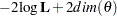
Let $\text{[math]}$ denote the dimension of the parameter vector $\text{[math]}$ . After the parameter estimation is completed, a table, called "Likelihood-Based Fit Statistics" is printed. It summarizes the likelihood calculations at $\text{[math]}$ . The first half of this table contains the information shown in Table 27.6.

Table 27.6 Likelihood Computation Summary
Statistic	Formula
Nonmissing response values used	$\text{[math]}$
Estimated parameters	$\text{[math]}$
Initialized diffuse state elements	$\text{[math]}$
Normalized residual sum of squares	$\text{[math]}$
Full log likelihood	$\text{[math]}$

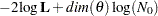
The second half of "Likelihood-Based Fit Statistics" table reports a variety of information-based criteria, which are functions of $\text{[math]}$ , $\text{[math]}$ , and $\text{[math]}$ . Table 27.7 summarizes the reported information criteria in smaller-is-better form:

Table 27.7 Information Criteria
Criterion	Formula	Reference
AIC	$\text{[math]}$	Akaike (1974)
AICC	$\text{[math]}$	Hurvich and Tsai (1989)
		Burnham and Anderson (1998)
HQIC	$\text{[math]}$	Hannan and Quinn (1979)
BIC	$\text{[math]}$	Schwarz (1978)
CAIC	$\text{[math]}$	Bozdogan (1987)

Forecasting Phase

After the model fitting phase, the filtering process is repeated again to produce the model-based one-step-ahead response variable forecasts ( $\text{[math]}$ ), residuals ( $\text{[math]}$ ), and their standard errors ( $\text{[math]}$ ). In addition, one-step-ahead forecasts of the components specified in the model statements, and any other user-defined linear combination of $\text{[math]}$ , are also produced. These forecasts are set to missing until the index $\text{[math]}$ (that is, until the filtering process is initialized). If the filtering process remains uninitialized, then all the one-step-ahead forecast related quantities, (such as $\text{[math]}$ and $\text{[math]}$ ) are reported as missing.

Smoothing Phase

After the filtering phase of KFS produces the one-step-ahead predictions of the response variables and the underlying state vectors, the smoothing phase of KFS produces the full-sample versions of these quantities—that is, rather than using the history up to $\text{[math]}$ , the entire sample $\text{[math]}$ is used. The smoothing phase of KFS is a backward algorithm, which begins at $\text{[math]}$ and $\text{[math]}$ and goes back towards $\text{[math]}$ and $\text{[math]}$ . It produces the following quantities:

Table 27.8 KFS: Smoothing Phase
$\text{[math]}$	Interpolated response value
$\text{[math]}$	Variance of the interpolated response value
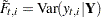
$\text{[math]}$	Full-sample estimate of the state vector
$\text{[math]}$	Covariance of $\text{[math]}$
$\text{[math]}$	Full-sample estimate of $\text{[math]}$ and $\text{[math]}$
$\text{[math]}$	Covariance of $\text{[math]}$
$\text{[math]}$	Estimate of additive outlier
$\text{[math]}$	Variance of $\text{[math]}$

Note that if $\text{[math]}$ is not missing, then 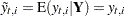$\text{[math]}$ and $\text{[math]}$ since, given $\text{[math]}$ , $\text{[math]}$ is completely known. Therefore, $\text{[math]}$ provides nontrivial information only when $\text{[math]}$ is missing—in which case $\text{[math]}$ represents the best estimate of $\text{[math]}$ based on the available data. The full sample estimates of components specified in the model equations are based on the corresponding linear combinations of $\text{[math]}$ . Similarly, their standard errors are computed by using appropriate functions of $\text{[math]}$ . The estimate of additive outlier, $\text{[math]}$ , is the difference between the observed response value $\text{[math]}$ and its estimate using all the data except $\text{[math]}$ , which is denoted by $\text{[math]}$ . The estimate $\text{[math]}$ is missing when $\text{[math]}$ is missing. For more information about the computation of additive outliers, see de Jong and Penzer (1998).

If the filtering process remains uninitialized until the end of the sample (that is, if $\text{[math]}$ is not invertible), some linear combinations of $\text{[math]}$ and $\text{[math]}$ are not estimable. This, in turn, implies that some linear combinations of $\text{[math]}$ are also inestimable. These inestimable quantities are reported as missing. For more information about the estimability of the state effects see Selukar (2010).

Note: This procedure is experimental.