The AUTOREG Procedure

Predicting the Unconditional Mean

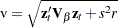
The first type of predicted value is obtained from only the structural part of the model, . These are useful in predicting values of new response time series, which are assumed to be described by the same model as the current response time series. The predicted values, residuals, and upper and lower confidence limits for the structural predictions are requested by specifying the PREDICTEDM=, RESIDUALM=, UCLM=, or LCLM= option in the OUTPUT statement. The ALPHACLM= option controls the confidence level for UCLM= and LCLM=. These confidence limits are for estimation of the mean of the dependent variable, , where is the column vector of independent variables at observation t.

The predicted values are computed as

and the upper and lower confidence limits as

where v is an estimate of the variance of and is the upper /2 percentage point of the t distribution.

where T is an observation from a t distribution with q degrees of freedom. The value of can be set with the ALPHACLM= option. The degrees of freedom parameter, q, is taken to be the number of observations minus the number of free parameters in the final model. For the YW estimation method, the value of v is calculated as

where is the error sum of squares divided by q. For the ULS and ML methods, it is calculated as

where is the submatrix of that corresponds to the regression parameters. For details, see the section Computational Methods earlier in this chapter.

Predicting Future Series Realizations

The other predicted values use both the structural part of the model and the predicted values of the error process. These conditional mean values are useful in predicting future values of the current response time series. The predicted values, residuals, and upper and lower confidence limits for future observations conditional on past values are requested by the PREDICTED=, RESIDUAL=, UCL=, or LCL= option in the OUTPUT statement. The ALPHACLI= option controls the confidence level for UCL= and LCL=. These confidence limits are for the predicted value,

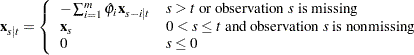
where is the vector of independent variables if all independent variables at time are nonmissing, and is the minimum variance linear predictor of the error term, which is defined in the following recursive way given the autoregressive model, AR(m) model, for :

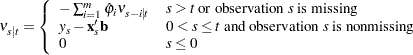where , are the estimated AR parameters. Observation is considered to be missing if the dependent variable or at least one independent variable is missing. If some of the independent variables at time are missing, the predicted is also missing. With the same definition of , the prediction method can be easily extended to the multistep forecast of :

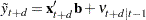The prediction method is implemented through the Kalman filter.

If is not missing, the upper and lower confidence limits are computed as

where v, in this case, is computed as

where is the variance-covariance matrix of the estimation of regression parameter ; is defined as

and is defined in a similar way as :

The value is the estimate of the conditional prediction error variance. At the start of the series, and after missing values, r is generally greater than 1. See the section Predicting the Conditional Variance for the computational details of r. The plot of residuals and confidence limits in Example 8.4 illustrates this behavior.

Except to adjust the degrees of freedom for the error sum of squares, the preceding formulas do not account for the fact that the autoregressive parameters are estimated. In particular, the confidence limits are likely to be somewhat too narrow. In large samples, this is probably not an important effect, but it might be appreciable in small samples. Refer to Harvey (1981) for some discussion of this problem for AR(1) models.

At the beginning of the series (the first m observations, where m is the value of the NLAG= option) and after missing values, these residuals do not match the residuals obtained by using OLS on the transformed variables. This is because, in these cases, the predicted noise values must be based on less than a complete set of past noise values and, thus, have larger variance. The GLS transformation for these observations includes a scale factor in addition to a linear combination of past values. Put another way, the matrix defined in the section Computational Methods has the value 1 along the diagonal, except for the first m observations and after missing values.

Predicting the Conditional Variance

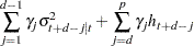
The GARCH process can be written

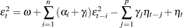where and . This representation shows that the squared residual follows an ARMA process. Then for any , the conditional expectations are as follows:

The d-step-ahead prediction error, = , has the conditional variance

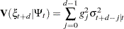where

Coefficients in the conditional d-step prediction error variance are calculated recursively using the formula

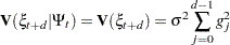
where and if ; , , are autoregressive parameters. Since the parameters are not known, the conditional variance is computed using the estimated autoregressive parameters. The d-step-ahead prediction error variance is simplified when there are no autoregressive terms:

Therefore, the one-step-ahead prediction error variance is equivalent to the conditional error variance defined in the GARCH process:

The multistep forecast of conditional error variance of the EGARCH, QGARCH, TGARCH, PGARCH, and GARCH-M models cannot be calculated using the preceding formula for the GARCH model. The following formulas are recursively implemented to obtain the multistep forecast of conditional error variance of these models:

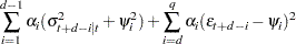
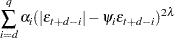
• for the EGARCH(p, q) model:

  where

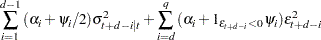
• for the QGARCH(p, q) model:

• for the TGARCH(p, q) model:

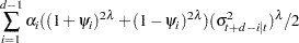
• for the PGARCH(p, q) model:

• for the GARCH-M model: ignoring the mean effect and directly using the formula of the corresponding GARCH model.

If the conditional error variance is homoscedastic, the conditional prediction error variance is identical to the unconditional prediction error variance

since . You can compute (which is the second term of the variance for the predicted value explained in the section Predicting Future Series Realizations) by using the formula , and r is estimated from by using the estimated autoregressive parameters.

Consider the following conditional prediction error variance:

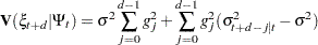The second term in the preceding equation can be interpreted as the noise from using the homoscedastic conditional variance when the errors follow the GARCH process. However, it is expected that if the GARCH process is covariance stationary, the difference between the conditional prediction error variance and the unconditional prediction error variance disappears as the forecast horizon d increases.