The AUTOREG Procedure
- Overview
-
Getting Started

-
Syntax
-
Details
Missing Values Autoregressive Error Model Alternative Autocorrelation Correction Methods GARCH Models Heteroscedasticity Consistent Covariance Matrix Estimator Goodness-of-Fit Measures and Information Criteria Testing Predicted Values OUT= Data Set OUTEST= Data Set Printed Output ODS Table Names ODS Graphics
-
Examples
- References
| Testing |
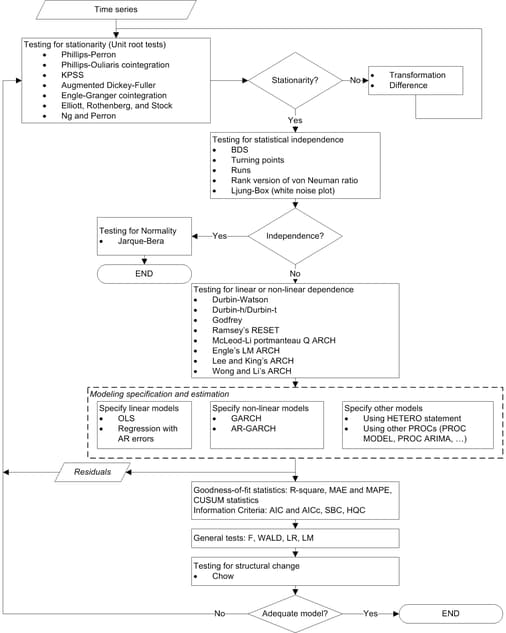
The modeling process consists of four stages: identification, specification, estimation, and diagnostic checking (Cromwell, Labys, and Terraza; 1994). The AUTOREG procedure supports tens of statistical tests for identification and diagnostic checking. Figure 8.15 illustrates how to incorporate these statistical tests into the modeling process.
Testing for Stationarity
Most of the theories of time series require stationarity; therefore, it is critical to determine whether a time series is stationary. Two nonstationary time series are fractionally integrated time series and autoregressive series with random coefficients. However, more often some time series are nonstationary due to an upward trend over time. The trend can be captured by either of the following two models.
-
The difference stationary process
where
 is the lag operator,
  , and
, and  is a white noise sequence with mean zero and variance
  . Hamilton (1994) also refers to this model the unit root process.
 -
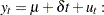
The trend stationary process

When a process has a unit root, it is said to be integrated of order one or I(1). An I(1) process is stationary after differencing once. The trend stationary process and difference stationary process require different treatment to transform the process into stationary one for analysis. Therefore, it is important to distinguish the two processes. Bhargava (1986) nested the two processes into the following general model
 |
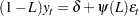
However, a difficulty is that the right-hand side is nonlinear in the parameters. Therefore, it is convenient to use a different parametrization
 |
The test of null hypothesis that  against the one-sided alternative of
  is called a unit root test.
Dickey-Fuller unit root tests are based on regression models similar to the previous model
 |
where is assumed to be white noise. The t statistic of the coefficient  does not follow the normal distribution asymptotically. Instead, its distribution can be derived using the functional central limit theorem. Three types of regression models including the preceding one are considered by the Dickey-Fuller test. The deterministic terms that are included in the other two types of regressions are either null or constant only.
An assumption in the Dickey-Fuller unit root test is that it requires the errors in the autoregressive model to be white noise, which is often not true. There are two popular ways to account for general serial correlation between the errors. One is the augmented Dickey-Fuller (ADF) test, which uses the lagged difference in the regression model. This was originally proposed by Dickey and Fuller (1979) and later studied by Said and Dickey (1984) and Phillips and Perron (1988). Another method is proposed by Phillips and Perron (1988); it is called Phillips-Perron (PP) test. The tests adopt the original Dickey-Fuller regression with intercept, but modify the test statistics to take account of the serial correlation and heteroscedasticity. It is called nonparametric because no specific form of the serial correlation of the errors is assumed.
A problem of the augmented Dickey-Fuller and Phillips-Perron unit root tests is that they are subject to size distortion and low power. It is reported in Schwert (1989) that the size distortion is significant when the series contains a large moving average (MA) parameter. DeJong et al. (1992) find that the ADF has power around one third and PP test has power less than 0.1 against the trend stationary alternative, in some common settings. Among some more recent unit root tests that improve upon the size distortion and the low power are the tests described by Elliott, Rothenberg, and Stock (1996) and Ng and Perron (2001). These tests involve a step of detrending before constructing the test statistics and are demonstrated to perform better than the traditional ADF and PP tests.
Most testing procedures specify the unit root processes as the null hypothesis. Tests of the null hypothesis of stationarity have also been studied, among which Kwiatkowski et al. (1992) is very popular.
Economic theories often dictate that a group of economic time series are linked together by some long-run equilibrium relationship. Statistically, this phenomenon can be modeled by cointegration. When several nonstationary processes 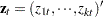 are cointegrated, there exists a
  cointegrating vector
  such that
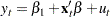
  is stationary and is a nonzero vector. One way to test the relationship of cointegration is the residual based cointegration test, which assumes the regression model
 |
where  ,
,  , and
, and  = (
= ( ,
, ,
, . The OLS residuals from the regression model are used to test for the null hypothesis of no cointegration. Engle and Granger (1987) suggest using ADF on the residuals while Phillips and Ouliaris (1990) study the tests using PP and other related test statistics.
Augmented Dickey-Fuller Unit Root and Engle-Granger Cointegration Testing
Common unit root tests have the null hypothesis that there is an autoregressive unit root  , and the alternative is
  , where is the autoregressive coefficient of the time series
 |
This is referred to as the zero mean model. The standard Dickey-Fuller (DF) test assumes that errors are white noise. There are two other types of regression models that include a constant or a time trend as follows:
 |
 |
|||
 |
 |
These two models are referred to as the constant mean model and the trend model, respectively. The constant mean model includes a constant mean  of the time series. However, the interpretation of depends on the stationarity in the following sense: the mean in the stationary case when is the trend in the integrated case when . Therefore, the null hypothesis should be the joint hypothesis that and
  . However for the unit root tests, the test statistics are concerned with the null hypothesis of . The joint null hypothesis is not commonly used. This issue is address in Bhargava (1986) with a different nesting model.
There are two types of test statistics. The conventional  ratio is
 |
and the second test statistic, called  -test, is
 |
For the zero mean model, the asymptotic distributions of the Dickey-Fuller test statistics are
 |
 |
|||
 |
 |
For the constant mean model, the asymptotic distributions are
|
 |
|||
|
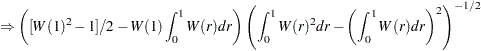 |
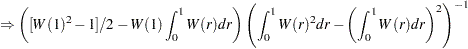
For the trend model, the asymptotic distributions are
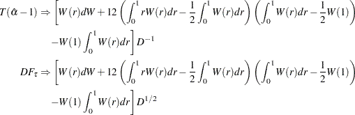 |
where
 |
One problem of the Dickey-Fuller and similar tests that employ three types of regressions is the difficulty in the specification of the deterministic trends. Campbell and Perron (1991) claimed that "the proper handling of deterministic trends is a vital prerequisite for dealing with unit roots". However the "proper handling" is not obvious since the distribution theory of the relevant statistics about the deterministic trends is not available. Hayashi (2000) suggests to using the constant mean model when you think there is no trend, and using the trend model when you think otherwise. However no formal procedure is provided.
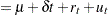
The null hypothesis of the Dickey-Fuller test is a random walk, possibly with drift. The differenced process is not serially correlated under the null of I(1). There is a great need for the generalization of this specification. The augmented Dickey-Fuller (ADF) test, originally proposed in Dickey and Fuller (1979), adjusts for the serial correlation in the time series by adding lagged first differences to the autoregressive model,
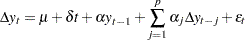 |
where the deterministic terms  and can be absent for the models without drift or linear trend. As previously, there are two types of test statistics. One is the OLS value
 |
and the other is given by
 |
The asymptotic distributions of the test statistics are the same as those of the standard Dickey-Fuller test statistics.
Nonstationary multivariate time series can be tested for cointegration, which means that a linear combination of these time series is stationary. Formally, denote the series by . The null hypothesis of cointegration is that there exists a vector such that is stationary. Residual-based cointegration tests were studied in Engle and Granger (1987) and Phillips and Ouliaris (1990). The latter are described in the next subsection. The first step regression is
 |
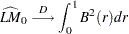
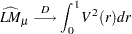
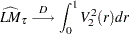
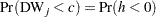
where ,  , and = (,,. This regression can also include an intercept or an intercept with a linear trend. The residuals are used to test for the existence of an autoregressive unit root. Engle and Granger (1987) proposed augmented Dickey-Fuller type regression without an intercept on the residuals to test the unit root. When the first step OLS does not include an intercept, the asymptotic distribution of the ADF test statistic
  is given by
 |
 |
|||
 |
 |
|||
 |
 |
|||
 |
 |
where  is a
is a  vector standard Brownian motion and
 |
is a partition such that  is a scalar and
  is
is  dimensional. The asymptotic distributions of the test statistics in the other two cases have the same form as the preceding formula. If the first step regression includes an intercept, then is replaced by the demeaned Brownian motion
 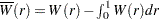 . If the first step regression includes a time trend, then is replaced by the detrended Brownian motion. The critical values of the asymptotic distributions are tabulated in Phillips and Ouliaris (1990) and MacKinnon (1991).
The residual based cointegration tests have a major shortcoming. Different choices of the dependent variable in the first step OLS might produce contradictory results. This can be explained theoretically. If the dependent variable is in the cointegration relationship, then the test is consistent against the alternative that there is cointegration. On the other hand, if the dependent variable is not in the cointegration system, the OLS residual  do not converge to a stationary process. Changing the dependent variable is more likely to produce conflicting results in finite samples.
Phillips-Perron Unit Root and Cointegration Testing
Besides the ADF test, there is another popular unit root test that is valid under general serial correlation and heteroscedasticity, developed by Phillips (1997) and Phillips and Perron (1988). The tests are constructed using the AR(1) type regressions, unlike ADF tests, with corrected estimation of the long run variance of  . In the case without intercept, consider the driftless random walk process
 |
where the disturbances might be serially correlated with possible heteroscedasticity. Phillips and Perron (1988) proposed the unit root test of the OLS regression model,
 |
Denote the OLS residual by  . The asymptotic variance of
  can be estimated by using the truncation lag l.
 |
where  ,
,  for
for  , and
, and 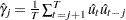 . This is a consistent estimator suggested by Newey and West (1987).
The variance of  can be estimated by
  . Let
. Let  be the variance estimate of the OLS estimator
  . Then the Phillips-Perron
  test (zero mean case) is written
 |
The statistic is just the ordinary Dickey-Fuller  statistic with a correction term that accounts for the serial correlation. The correction term goes to zero asymptotically if there is no serial correlation.
Note that  as
as  , which shows that the limiting distribution is skewed to the left.
Let  be the
  statistic for . The Phillips-Perron
  (defined here as
  ) test is written
 |
To incorporate a constant intercept, the regression model  is used (single mean case) and null hypothesis the series is a driftless random walk with nonzero unconditional mean. To incorporate a time trend, we used the regression model
  and under the null the series is a random walk with drift.
The limiting distributions of the test statistics for the zero mean case are
 |
 |
|||
 |
 |
where B( ) is a standard Brownian motion.
The limiting distributions of the test statistics for the intercept case are
 |
 |
|||
 |
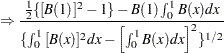 |
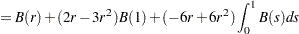
Finally, The limiting distributions of the test statistics for the trend case are can be derived as
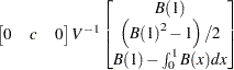 |
where  for
for  and
and  for ,
for ,
 |
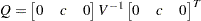 |
The finite sample performance of the PP test is not satisfactory ( see Hayashi (2000) ).
When several variables are cointegrated, there exists a cointegrating vector such that is stationary and is a nonzero vector. The residual based cointegration test assumes the following regression model:
|
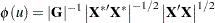
where , , and = (,,. You can estimate the consistent cointegrating vector by using OLS if all variables are difference stationary — that is, I(1). The estimated cointegrating vector is 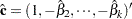 . The Phillips-Ouliaris test is computed using the OLS residuals from the preceding regression model, and it uses the PP unit root tests
  and
and  developed in Phillips (1997), although in Phillips and Ouliaris (1990) the asymptotic distributions of some other leading unit root tests are also derived. The null hypothesis is no cointegration.
You need to refer to the tables by Phillips and Ouliaris (1990) to obtain the  -value of the cointegration test. Before you apply the cointegration test, you may want to perform the unit root test for each variable (see the option STATIONARITY=( ADF)).
As in the Engle-Granger cointegration tests, the Phillips-Ouliaris test can give conflicting results for different choices of the regressand. There are other cointegration tests that are invariant to the order of the variables, including Johansen (1988), Johansen (1991), Stock and Watson (1988).
ERS and Ng-Perron Unit Root Tests
(Experimental)As mentioned earlier, ADF and PP both suffer severe size distortion and low power. There is a class of newer tests that improves both size and power, sometimes called efficient unit root tests, among which Elliott, Rothenberg, and Stock (1996) and Ng and Perron (2001) are prominent.
Elliott, Rothenberg, and Stock (1996) consider the data generating process
|
 |
|||
 |
 |
where  is either
  or
or  and
and  is an unobserved stationary zero-mean process with positive spectral density at zero frequency. The null hypothesis is , and the alternative is . The key idea of Elliott, Rothenberg, and Stock (1996) is to study the asymptotic power and asymptotic power envelope of some new tests. Asymptotic power is defined with a sequence of local alternatives. For a fixed alternative hypothesis, the power of a test usually goes to one when sample size goes to infinity; however, this does not say anything about the finite sample performance. On the other hand, when the data generating process under the alternative moves closer to the null as the sample size increases, the power does not necessarily converge to one. The local to unity alternatives in ERS are
 |
and the power against the local alternatives has a limit as  goes to infinity, which is called asymptotic power. This value is strictly between 0 and 1. Asymptotic power indicates the adequacy of a test to distinguish small deviations from the null hypothesis.
Define
 |
 |
|||
 |
 |
Let  be the sum of squared residuals from a least squares regression of
  on
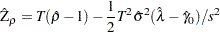
on  . Then the point optimal test against the local alternative
  has the form
 |
where  is an estimator for
  . Note that the test rejects the null when
  is small. The asymptotic power function for the point optimal test constructed with
  under local alternatives with
  is denoted by
  . Then the power envelope is
  because the test formed with is the most powerful against the alternative
  . In other words, the asymptotic function
  , is always below the power envelope
  except that at one point they are tangent. Elliott, Rothenberg, and Stock (1996) show that choosing some specific values for can cause the asymptotic power function of the point optimal test to be very close to the power envelope. The optimal is
  when
when  , and
, and  when
when  . This choice of corresponds to the tangent point where
  . This is also true for the DF-GLS test.
Elliott, Rothenberg, and Stock (1996) also propose the DF-GLS test, given by the statistic for testing  in the regression
 |
where  is obtained in a first step detrending
 |
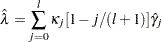
and  is least squares regression coefficient of on . Regarding the lag length selection, Elliott, Rothenberg, and Stock (1996) favor the Schwartz Bayesian information criterion. The optimal selection of the lag length and the estimation of
  is further discussed in Ng and Perron (2001). The lag length is selected from the interval
  for some fixed
  by using the modified Akaike’s information criterion,
 |
where  and
and 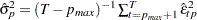 . For fixed lag length , an estimate of is given by
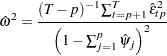 |
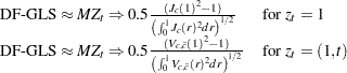
DF-GLS is indeed a superior unit root test, according to Stock (1994), Schwert (1989), and Elliott, Rothenberg, and Stock (1996). In terms of the size of the test, DF-GLS is almost as good as the ADF test  and better than the PP
  and
and  test. In addition, the power of the DF-GLS is larger than the ADF test and -test.
Ng and Perron (2001) also apply GLS detrending to obtain the following M-tests:
 |
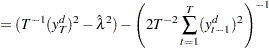 |
|||
 |
 |
|||
 |
 |
The first one is a modified version of Phillips-Perron  test
test
 |
where the detrended data  is used. The second is a modified Bhargava (1986)
  test statistic. The third can be perceived as a modified Phillips-Perron
  statistic because of the relationship
  .
.
The modified point optimal tests using the GLS detrended data are
 |
The DF-GLS test and the  test have the same limiting distribution
 |
The point optimal test and the modified point optimal test have the same limiting distribution
 |
where is a standard Brownian motion and  is an Ornstein-Uhlenbeck process defined by
  with
with  ,
,  , and
, and 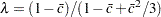 .
.
Overall, the M-tests has the smallest size distortion, with the ADF t test having the next smallest. The ADF -test, , and have the worst size distortion. In addition, the power of the DF-GLS and M-tests are larger than that of the ADF t test and -test. The ADF has more severe size distortion than the ADF , but larger power for a fixed lag length.
Kwiatkowski, Phillips, Schmidt, and Shin (KPSS) Unit Root Test
There are less existent tests for the null hypothesis of trend stationary I(0). The main reason is the difficulty in the theoretical development. The KPSS test was introduced in Kwiatkowski et al. (1992) to test the null hypothesis that an observable series is stationary around a deterministic trend. Please note, that for consistency reasons, the notation used here is different from the notation used in the original paper. The setup of the problem is as follows: it is assumed that the series is expressed as the sum of the deterministic trend, random walk  , and stationary error ; that is,
|
 |
|||
 |
 |
where  iid
iid  , and an intercept (in the original paper, the authors use
  instead of , here we assume
  .) The null hypothesis of trend stationary is specified by
  , while the null of level stationary is the same as above with the model restriction
  . Under the alternative that
  , there is a random walk component in the observed series
  .
.
Under stronger assumptions of normality and iid of and  , a one-sided LM test of the null that there is no random walk (
 ) can be constructed as follows:
 |
 |
|||
 |
 |
|||
 |
 |
Notice that under the null hypothesis,  can be estimated by ordinary least squares regression of on an intercept and the time trend. Following the original work of Kwiatkowski, Phillips, Schmidt, and Shin, under the null (
 ),
),  statistic converges asymptotically to three different distributions depending on whether the model is trend-stationary, level-stationary (
 ), or zero-mean stationary (,
  ). The trend-stationary model is denoted by subscript and the level-stationary model is denoted by subscript . The case when there is no trend and zero intercept is denoted as 0. The last case, although rarely used in practice, is considered in Hobijn, Franses, and Ooms (2004).
 |
 |
|||
 |
 |
|||
 |
 |
with
 |
 |
|||
 |
 |
where  is a Brownian motion (Wiener process), and
  is convergence in distribution. Note that
  is a standard Brownian bridge,
  is a Brownian bridge of a second-level.
Using the notation of Kwiatkowski et al. (1992) the  statistic is named as
  . This test depends on the computational method used to compute the long-run variance
  — that is, the window width
  and the kernel type
  . You can specify the kernel used in the test, using the KERNEL option:
-
Newey-West/Bartlett (KERNEL=NW
 BART), default
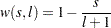
-
Quadratic spectral (KERNEL=QS)

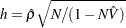
You can specify the number of lags, , in three different ways:
-
Schwert (SCHW = c) (default for NW, c=4)
Manual (LAG =
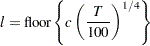
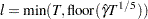
) Automatic selection (AUTO) (default for QS) Hobijn, Franses, and Ooms (2004)
The last option (AUTO) needs more explanation, summarized in the following table. For each of the kernel function, a formula for optimal window width is provided.
NW Kernel |
QS Kernel |
||
|---|---|---|---|
|
|
||
where |
|||
|
|
||
|
|||
|
|
||


where  if
if  and 0, otherwise;
  .
.
Simulation evidence shows that the KPSS has size distortion in finite samples. For example, see Caner and Kilian (2001). The power is reduced when the sample size is large, which can be derived theoretically (see Breitung (1995)). Another problem of the KPSS test is that the power depends on the choice of the truncation lag used in the Newey-West estimator of the long run variance  .
.
Testing for Statistical Independence
Independence tests are widely used in model selection, residual analysis, and model diagnostics because models are usually based on the assumption of independently distributed errors. If a given time series (for example, a series of residuals) is independent, then no determinic model is necessary for this completely random process; otherwise, there must exist some relationship in the series to be addressed. In the following section, four independence tests are introduced: the BDS test, the runs test, the turning point test, and the rank version of von Neumann ratio test.
BDS Test
Broock, Dechert, and Scheinkman (1987) propose a test (BDS test) of independence based on the correlation dimension. Broock et al. (1996) show that the first-order asymptotic distribution of the test statistic is independent of the estimation error provided that the parameters of the model under test can be estimated  -consistently. Hence, the BDS test can be used as a model selection tool and as a specification test.
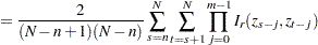
Given the sample size , the embedding dimension  , and the value of the radius
  , the BDS statistic is
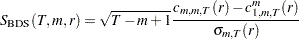 |
where
 |
 |
|||
 |
 |
|||
 |
 |
|||
 |
 |
|||
 |
 |
|||
 |
 |
The statistic has a standard normal distribution if the sample size is large enough. For small sample size, the distribution can be approximately obtained through simulation. Kanzler (1999) has a comprehensive discussion on the implementation and empirical performance of BDS test.
Runs Test and Turning Point Test
The runs test and turning point test are two widely used tests for independence (Cromwell, Labys, and Terraza; 1994).
The runs test needs several steps. First, convert the original time series into the sequence of signs,  , that is, map into
  where
where  is the sample mean of
  and
and  is "
is " " if
" if  is nonnegative and "
 " if is negative. Second, count the number of runs,
  , in the sequence. A run of a sequence is a maximal non-empty segment of the sequence that consists of adjacent equal elements. For example, the following sequence contains
  runs:
runs:
 |
Third, count the number of pluses and minuses in the sequence and denote them as  and
and  , respectively. In the preceding example sequence,
  and
and  . Note that the sample size
  . Finally, compute the statistic of runs test,
 |
where
 |
 |
The statistic of the turning point test is defined as follows:
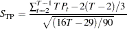 |
where the indicator function of the turning point  is 1 if
  or
or  (that is, both the previous and next values are greater or less than the current value); otherwise, 0.
The statistics of both the runs test and the turning point test have the standard normal distribution under the null hypothesis of independence.
Rank Version of von Neumann Ratio Test
Since the runs test completely ignores the magnitudes of the observations, Bartels (1982) proposes a rank version of the von Neumann Ratio test for independence:
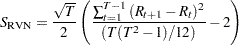 |
where  is the rank of th observation in the sequence of observations. For large sample, the statistic follows the standard normal distribution under the null hypothesis of independence. For small samples of size between 11 and 100, the critical values through simulation would be more precise; for samples of size no more than 10, the exact CDF is applied.
Testing for Normality
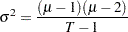
Based on skewness and kurtosis, Jarque and Bera (1980) calculated the test statistic
 |
where
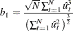 |
 |
The 
 (2) distribution gives an approximation to the normality test
  .
.
When the GARCH model is estimated, the normality test is obtained using the standardized residuals  . The normality test can be used to detect misspecification of the family of ARCH models.
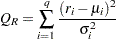
Testing for Linear Dependence
Generalized Durbin-Watson Tests
Consider the following linear regression model:
 |
where  is an
is an  data matrix,
  is a
is a  coefficient vector, and
  is a
is a  disturbance vector. The error term is assumed to be generated by the
  th-order autoregressive process
  where
where  ,
,  is a sequence of independent normal error terms with mean 0 and variance
  . Usually, the Durbin-Watson statistic is used to test the null hypothesis
  against
  . Vinod (1973) generalized the Durbin-Watson statistic:
 |
where  are OLS residuals. Using the matrix notation,
 |
where 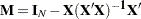 and
and  is a
is a  matrix:
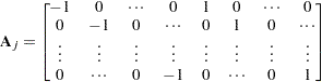 |
and there are  zeros between
  and 1 in each row of matrix
  .
.
The QR factorization of the design matrix yields a  orthogonal matrix
  :
:
 |
where R is an upper triangular matrix. There exists an  submatrix of such that
  and
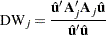
and  . Consequently, the generalized Durbin-Watson statistic is stated as a ratio of two quadratic forms:
 |
where  are upper n eigenvalues of
  and
and  is a standard normal variate, and
  . These eigenvalues are obtained by a singular value decomposition of
  (Golub and Van Loan; 1989; Savin and White; 1978).
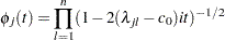
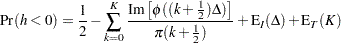
The marginal probability (or p-value) for  given
given  is
is
 |
where
 |
When the null hypothesis  holds, the quadratic form
  has the characteristic function
 |
The distribution function is uniquely determined by this characteristic function:
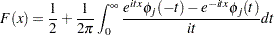 |
For example, to test  given
given 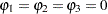 against
  , the marginal probability (p-value) can be used:
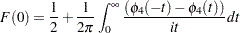 |
where
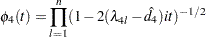 |
and  is the calculated value of the fourth-order Durbin-Watson statistic.
In the Durbin-Watson test, the marginal probability indicates positive autocorrelation ( ) if it is less than the level of significance (
 ), while you can conclude that a negative autocorrelation (
 ) exists if the marginal probability based on the computed Durbin-Watson statistic is greater than
  . Wallis (1972) presented tables for bounds tests of fourth-order autocorrelation, and Vinod (1973) has given tables for a 5% significance level for orders two to four. Using the AUTOREG procedure, you can calculate the exact p-values for the general order of Durbin-Watson test statistics. Tests for the absence of autocorrelation of order p can be performed sequentially; at the th step, test given
  against
  . However, the size of the sequential test is not known.
The Durbin-Watson statistic is computed from the OLS residuals, while that of the autoregressive error model uses residuals that are the difference between the predicted values and the actual values. When you use the Durbin-Watson test from the residuals of the autoregressive error model, you must be aware that this test is only an approximation. See Autoregressive Error Model earlier in this chapter. If there are missing values, the Durbin-Watson statistic is computed using all the nonmissing values and ignoring the gaps caused by missing residuals. This does not affect the significance level of the resulting test, although the power of the test against certain alternatives may be adversely affected. Savin and White (1978) have examined the use of the Durbin-Watson statistic with missing values.
The Durbin-Watson probability calculations have been enhanced to compute the -value of the generalized Durbin-Watson statistic for large sample sizes. Previously, the Durbin-Watson probabilities were only calculated for small sample sizes.
Consider the following linear regression model:
 |
 |
where is an  data matrix, is a
  coefficient vector,
  is a
is a  disturbance vector, and is a sequence of independent normal error terms with mean 0 and variance .
The generalized Durbin-Watson statistic is written as
 |
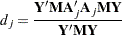
where  is a vector of OLS residuals and
  is a
is a  matrix. The generalized Durbin-Watson statistic DW
 can be rewritten as
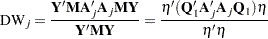 |
where  .
.
The marginal probability for the Durbin-Watson statistic is
 |
where  .
.
The -value or the marginal probability for the generalized Durbin-Watson statistic is computed by numerical inversion of the characteristic function  of the quadratic form . The trapezoidal rule approximation to the marginal probability
  is
is
 |
where  is the imaginary part of the characteristic function,
  and
and  are integration and truncation errors, respectively. Refer to Davies (1973) for numerical inversion of the characteristic function.
Ansley, Kohn, and Shively (1992) proposed a numerically efficient algorithm that requires O( ) operations for evaluation of the characteristic function . The characteristic function is denoted as
 |
 |
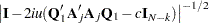 |
|||
 |
|
 |
where 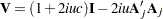 and
and  . By applying the Cholesky decomposition to the complex matrix
  , you can obtain the lower triangular matrix
  that satisfies
  . Therefore, the characteristic function can be evaluated in O() operations by using the following formula:
 |
where  . Refer to Ansley, Kohn, and Shively (1992) for more information on evaluation of the characteristic function.
Tests for Serial Correlation with Lagged Dependent Variables
When regressors contain lagged dependent variables, the Durbin-Watson statistic ( ) for the first-order autocorrelation is biased toward 2 and has reduced power. Wallis (1972) shows that the bias in the Durbin-Watson statistic (
 ) for the fourth-order autocorrelation is smaller than the bias in in the presence of a first-order lagged dependent variable. Durbin (1970) proposes two alternative statistics (Durbin h and t ) that are asymptotically equivalent. The h statistic is written as
 |
where  and
and  is the least squares variance estimate for the coefficient of the lagged dependent variable. Durbin’s t test consists of regressing the OLS residuals
  on explanatory variables and
  and testing the significance of the estimate for coefficient of .
Inder (1984) shows that the Durbin-Watson test for the absence of first-order autocorrelation is generally more powerful than the h test in finite samples. Refer to Inder (1986) and King and Wu (1991) for the Durbin-Watson test in the presence of lagged dependent variables.
Godfrey LM test
The GODFREY= option in the MODEL statement produces the Godfrey Lagrange multiplier test for serially correlated residuals for each equation (Godfrey 1978a and 1978b). is the maximum autoregressive order, and specifies that Godfrey’s tests be computed for lags 1 through . The default number of lags is four.
Testing for Nonlinear Dependence: Ramsey’s Reset Test
Ramsey’s reset test is a misspecification test associated with the functional form of models to check whether power transforms need to be added to a model. The original linear model, henceforth called the restricted model, is
 |
To test for misspecification in the functional form, the unrestricted model is
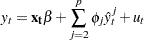 |
where  is the predicted value from the linear model and is the power of in the unrestricted model equation starting from 2. The number of higher-ordered terms to be chosen depends on the discretion of the analyst. The RESET option produces test results for
  2, 3, and 4.
The reset test is an F statistic for testing  , for all
  , against
  for at least one in the unrestricted model and is computed as follows:
 |
where  is the sum of squared errors due to the restricted model,
  is the sum of squared errors due to the unrestricted model,
  is the total number of observations, and is the number of parameters in the original linear model.
Ramsey’s test can be viewed as a linearity test that checks whether any nonlinear transformation of the specified independent variables has been omitted, but it need not help in identifying a new relevant variable other than those already specified in the current model.
Testing for Nonlinear Dependence: Heteroscedasticity Tests
Portmanteau Q Test
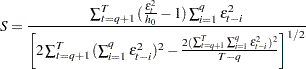
For nonlinear time series models, the portmanteau test statistic based on squared residuals is used to test for independence of the series (McLeod and Li; 1983):
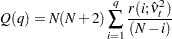 |
where
 |
 |
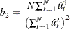
This Q statistic is used to test the nonlinear effects (for example, GARCH effects) present in the residuals. The GARCH process can be considered as an ARMA
 process. See the section Predicting the Conditional Variance. Therefore, the Q statistic calculated from the squared residuals can be used to identify the order of the GARCH process.
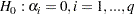
Engle’s Lagrange Multiplier Test for ARCH Disturbances
Engle (1982) proposed a Lagrange multiplier test for ARCH disturbances. The test statistic is asymptotically equivalent to the test used by Breusch and Pagan (1979). Engle’s Lagrange multiplier test for the qth order ARCH process is written
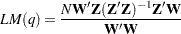 |
where
 |
and
 |
The presample values (  ,
, ,
,  ) have been set to 0. Note that the LM
 tests might have different finite-sample properties depending on the presample values, though they are asymptotically equivalent regardless of the presample values.
Lee and King’s Test for ARCH Disturbances
Engle’s Lagrange multiplier test for ARCH disturbances is a two-sided test; that is, it ignores the inequality constraints for the coefficients in ARCH models. Lee and King (1993) propose a one-sided test and prove that the test is locally most mean powerful. Let  , denote the residuals to be tested. Lee and King’s test checks
 |
 |
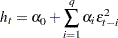
where  are in the following ARCH(q) model:
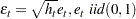 |
 |
The statistic is written as
 |
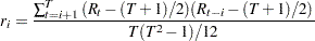
Wong and Li’s Test for ARCH Disturbances
Wong and Li (1995) propose a rank portmanteau statistic to minimize the effect of the existence of outliers in the test for ARCH disturbances. They first rank the squared residuals; that is,  . Then they calculate the rank portmanteau statistic
 |
where  ,
,  , and
, and  are defined as follows:
 |
 |
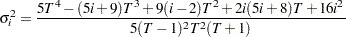 |
The Q, Engle’s LM, Lee and King’s, and Wong and Li’s statistics are computed from the OLS residuals, or residuals if the NLAG= option is specified, assuming that disturbances are white noise. The Q, Engle’s LM, and Wong and Li’s statistics have an approximate  distribution under the white-noise null hypothesis, while the Lee and King’s statistic has a standard normal distribution under the white-noise null hypothesis.
Testing for Structural Change: Chow Test
Consider the linear regression model
 |
where the parameter vector contains elements.
Split the observations for this model into two subsets at the break point specified by the CHOW= option, so that
 |
|
 |
|||
 |
|
 |
|||
 |
|
 |
Now consider the two linear regressions for the two subsets of the data modeled separately,
 |
 |
where the number of observations from the first set is  and the number of observations from the second set is
  .
.
The Chow test statistic is used to test the null hypothesis  conditional on the same error variance
  . The Chow test is computed using three sums of square errors:
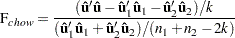 |
where  is the regression residual vector from the full set model,
  is the regression residual vector from the first set model, and
  is the regression residual vector from the second set model. Under the null hypothesis, the Chow test statistic has an F distribution with
  and
and  degrees of freedom, where is the number of elements in
  .
.
Chow (1960) suggested another test statistic that tests the hypothesis that the mean of prediction errors is 0. The predictive Chow test can also be used when  .
.
The PCHOW= option computes the predictive Chow test statistic
 |
The predictive Chow test has an F distribution with and  degrees of freedom.