| The UCM Procedure |
Example 31.6 Using Splines to Incorporate Nonlinear Effects
The data in this example are created to mirror the electricity demand and temperature data recorded at a utility company in the midwest region of the United States. The data set (not shown), utility, has three variables: load, temp, and date. The load column contains the daily electricity demand, the temp column has the average daily temperature readings, and the date column records the observation date.
The following statements produce a plot, shown in Output 31.6.1, of electricity load versus temperature. Clearly the relationship is smooth but nonlinear: the load generally increases when the temperatures are away from the comfortable sixties.
ods graphics on;
proc sgplot data=utility;
    loess x=temp y=load / smooth=0.4;
run;
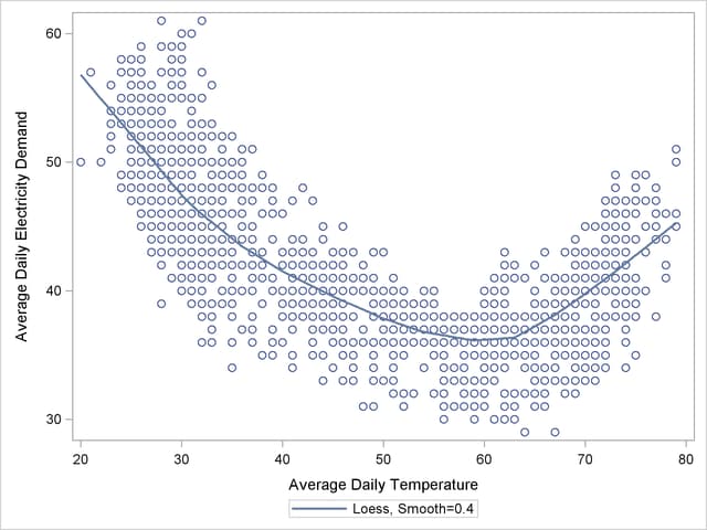
The time series plot of the load (not shown) also shows that, apart from a day-of-the-week seasonal effect, there are no additional easily identifiable patterns in the series. The series has no apparent upward or downward trend. The following statements fit a UCM to the series that takes into account these observations. The particular choice of the model is a result of a little modeling exercise that compared a small number of competing models. The chosen model is adequate but by no means the best possible. The temperature effect is modeled by a deterministic three-degree spline with knots at 30, 40, 50, 60, and 75. The knot locations and the degree were chosen by visual inspection of the plot (Output 31.6.1). An autoreg component is used in place of the simple irregular component, which improved the residual analysis. The last 60 days of data are withheld for out-of-sample forecast evaluation (note the BACK= option in both the ESTIMATE and FORECAST statements). The OUTLIER statement is used to increase the number of outliers reported to 10. Since no CHECKBREAK option is used in the LEVEL statement, only the additive outliers are searched. In this example the use of the EXTRADIFFUSE= option in the ESTIMATE and FORECAST statements is useful for discarding some early one-step-ahead forecasts and residuals with large variance.
proc ucm data=utility;
   id date interval=day;
   model load;
   autoreg;
   level plot=smooth;
   splinereg temp knots=30 40 50 65 75 degree=3
      variance=0 noest;
   season length=7 var=0 noest;
      estimate plot=panel back=60
      extradiffuse=50;
   outlier maxnum=10;
   forecast back=60 lead=60
      extradiffuse=50;
run;
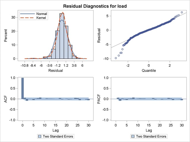
The parameter estimates are given in Output 31.6.2, and the residual goodness-of-fit statistics are shown in Output 31.6.3. The residual diagnostic plots are shown in Output 31.6.4. The ACF and PACF plots appear satisfactory, but the normality plots, particularly the Q-Q plot, show possible violations. It appears that, at least in part, this nonNormal behavior of the residuals might be attributable to the outliers in the series. The outlier summary table, Output 31.6.5, shows the most likely outlying observations. Notice that most of these outliers are holidays, like July 4th, when the electricity load is lower than usual for that day of the week.
| Final Estimates of the Free Parameters | |||||
|---|---|---|---|---|---|
| Component | Parameter | Estimate | Approx Std Error |
t Value | Approx Pr > |t| |
| Level | Error Variance | 0.21185 | 0.05025 | 4.22 | <.0001 |
| AutoReg | Damping Factor | 0.57522 | 0.03466 | 16.60 | <.0001 |
| AutoReg | Error Variance | 2.21057 | 0.20478 | 10.79 | <.0001 |
| temp | Spline Coefficient_1 | 4.72502 | 1.93997 | 2.44 | 0.0149 |
| temp | Spline Coefficient_2 | 2.19116 | 1.71243 | 1.28 | 0.2007 |
| temp | Spline Coefficient_3 | -7.14492 | 1.56805 | -4.56 | <.0001 |
| temp | Spline Coefficient_4 | -11.39950 | 1.45098 | -7.86 | <.0001 |
| temp | Spline Coefficient_5 | -16.38055 | 1.36977 | -11.96 | <.0001 |
| temp | Spline Coefficient_6 | -18.76075 | 1.28898 | -14.55 | <.0001 |
| temp | Spline Coefficient_7 | -8.04628 | 1.09017 | -7.38 | <.0001 |
| temp | Spline Coefficient_8 | -2.30525 | 1.25102 | -1.84 | 0.0654 |
| Fit Statistics Based on Residuals | |
|---|---|
| Mean Squared Error | 2.90945 |
| Root Mean Squared Error | 1.70571 |
| Mean Absolute Percentage Error | 2.92586 |
| Maximum Percent Error | 14.96281 |
| R-Square | 0.92739 |
| Adjusted R-Square | 0.92721 |
| Random Walk R-Square | 0.69618 |
| Amemiya's Adjusted R-Square | 0.92684 |
| Number of non-missing residuals used for computing the fit statistics = 791 | |
| Obs | Time | Estimate | StdErr | ChiSq | DF | ProbChiSq |
|---|---|---|---|---|---|---|
| 1281 | 04JUL2002 | -7.99908 | 1.3417486 | 35.54 | 1 | <.0001 |
| 916 | 04JUL2001 | -6.55778 | 1.338431 | 24.01 | 1 | <.0001 |
| 329 | 25NOV1999 | -5.85047 | 1.3379735 | 19.12 | 1 | <.0001 |
| 977 | 03SEP2001 | -5.67254 | 1.3389138 | 17.95 | 1 | <.0001 |
| 1341 | 02SEP2002 | -5.49631 | 1.337843 | 16.88 | 1 | <.0001 |
| 693 | 23NOV2000 | -5.27968 | 1.3374368 | 15.58 | 1 | <.0001 |
| 915 | 03JUL2001 | 5.06557 | 1.3375273 | 14.34 | 1 | 0.0002 |
| 1057 | 22NOV2001 | -5.01550 | 1.3386184 | 14.04 | 1 | 0.0002 |
| 551 | 04JUL2000 | -4.89965 | 1.3381557 | 13.41 | 1 | 0.0003 |
| 879 | 28MAY2001 | -4.76135 | 1.3375349 | 12.67 | 1 | 0.0004 |
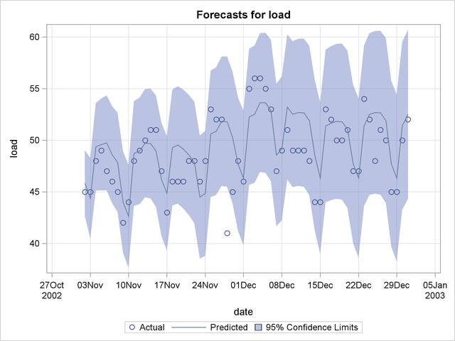
The plot of the load forecasts for the withheld data is shown in Output 31.6.6.
Copyright © SAS Institute, Inc. All Rights Reserved.