| The COUNTREG Procedure |
Example 10.2 ZIP and ZINB Models for Data Exhibiting Extra Zeros
In the study by Long (1997) of the number of published articles by scientists (see the section Getting Started: COUNTREG Procedure), the observed proportion of scientists publishing no articles is 0.3005. The following statements use PROC FREQ to compute the proportion of scientists publishing each observed number of articles. Output 10.2.1 shows the results.
    proc freq data=long97data;
       table art / out=obs;
    run;
| art | Frequency | Percent | Cumulative Frequency |
Cumulative Percent |
|---|---|---|---|---|
| 0 | 275 | 30.05 | 275 | 30.05 |
| 1 | 246 | 26.89 | 521 | 56.94 |
| 2 | 178 | 19.45 | 699 | 76.39 |
| 3 | 84 | 9.18 | 783 | 85.57 |
| 4 | 67 | 7.32 | 850 | 92.90 |
| 5 | 27 | 2.95 | 877 | 95.85 |
| 6 | 17 | 1.86 | 894 | 97.70 |
| 7 | 12 | 1.31 | 906 | 99.02 |
| 8 | 1 | 0.11 | 907 | 99.13 |
| 9 | 2 | 0.22 | 909 | 99.34 |
| 10 | 1 | 0.11 | 910 | 99.45 |
| 11 | 1 | 0.11 | 911 | 99.56 |
| 12 | 2 | 0.22 | 913 | 99.78 |
| 16 | 1 | 0.11 | 914 | 99.89 |
| 19 | 1 | 0.11 | 915 | 100.00 |
PROC COUNTREG is then used to fit Poisson and negative binomial models to the data. For each model, the PROBCOUNTS macro computes the probability that the number of published articles is  , where is a value in a list of nonnegative integers specified in the COUNTS= option. The computations require the parameter estimates of the fitted model. These are saved using the ODS OUTPUT statement as shown and passed to the PROBCOUNTS macro by using the INMODEL= option. Variables containing the probabilities are created with names beginning with the PREFIX= string followed by the COUNTS= values and are saved in the OUT= data set. For the Poisson model, the variables poi0, poi1,
  , poi10 are created and saved in the data set predpoi, which also contains all of the variables in the DATA= data set. The PROBCOUNTS macro is available from the Samples section at http://support.sas.com. The following statements compute the estimates for Poisson and negative binomial models.
    /*-- Poisson Model --*/
    proc countreg data=long97data;
       model art=fem mar kid5 phd ment / dist=poisson;
       ods output ParameterEstimates=pe;
    run;

    %include probcounts;
    %probcounts(data=long97data,
                inmodel=pe,
                counts=0 to 10,
                prefix=poi, out=predpoi)

    /*-- Negative Binomial Model --*/
    proc countreg data=long97data;
       model art=fem mar kid5 phd ment / dist=negbin(p=2);
       ods output ParameterEstimates=pe;
    run;

    %probcounts(data=predpoi,
                inmodel=pe,
                counts=0 to 10,
                prefix=nb, out=prednb)
Parameter estimates for these two models are shown in the section Getting Started: COUNTREG Procedure. For each model, the predicted proportion of zero articles can be calculated as the average predicted probability of zero articles across all scientists as shown in the macro probcounts in the following program. Under the Poisson model, the predicted proportion of zero articles is 0.2092, which considerably underestimates the observed proportion. The negative binomial more closely estimates the proportion of zeros (0.3036). Also, the test of the dispersion parameter, _Alpha, in the negative binomial model indicates significant overdispersion ( ). As a result, the negative binomial model is preferred to the Poisson model.
Another way to account for the large number of zeros in this data set is to fit a zero-inflated Poisson (ZIP) or a zero-inflated negative binomial (ZINB) model. In the following statements, DIST=ZIP requests the ZIP model. In the ZEROMODEL statement, you can specify the predictors,  , for the process that generated the additional zeros. The ZEROMODEL statement also specifies the model for the probability
  . By default, a logistic model is used for . The default can be changed using the LINK= option. In this particular ZIP model, all variables used to model the article counts are also used to model .
    proc countreg data=long97data;
       model art = fem mar kid5 phd ment / dist=zip;
       zeromodel art ~ fem mar kid5 phd ment;
       ods output ParameterEstimates=pe;
    run;

    %probcounts(data=prednb,
                inmodel=pe,
                counts=0 to 10,
                prefix=zip, out=predzip)
The parameters of the ZIP model are displayed in Output 10.2.2. The first set of parameters gives the estimates of  in the model for the Poisson process mean. Parameters with the prefix "Inf_" are the estimates of
  in the logistic model for .
| Model Fit Summary | |
|---|---|
| Dependent Variable | art |
| Number of Observations | 915 |
| Data Set | WORK.LONG97DATA |
| Model | ZIP |
| ZI Link Function | Logistic |
| Log Likelihood | -1605 |
| Maximum Absolute Gradient | 2.08803E-7 |
| Number of Iterations | 16 |
| Optimization Method | Newton-Raphson |
| AIC | 3234 |
| SBC | 3291 |
| Parameter Estimates | |||||
|---|---|---|---|---|---|
| Parameter | DF | Estimate | Standard Error | t Value | Approx Pr > |t| |
| Intercept | 1 | 0.640838 | 0.121306 | 5.28 | <.0001 |
| fem | 1 | -0.209145 | 0.063405 | -3.30 | 0.0010 |
| mar | 1 | 0.103751 | 0.071111 | 1.46 | 0.1446 |
| kid5 | 1 | -0.143320 | 0.047429 | -3.02 | 0.0025 |
| phd | 1 | -0.006166 | 0.031008 | -0.20 | 0.8424 |
| ment | 1 | 0.018098 | 0.002295 | 7.89 | <.0001 |
| Inf_Intercept | 1 | -0.577060 | 0.509383 | -1.13 | 0.2573 |
| Inf_fem | 1 | 0.109747 | 0.280082 | 0.39 | 0.6952 |
| Inf_mar | 1 | -0.354013 | 0.317611 | -1.11 | 0.2650 |
| Inf_kid5 | 1 | 0.217101 | 0.196481 | 1.10 | 0.2692 |
| Inf_phd | 1 | 0.001272 | 0.145262 | 0.01 | 0.9930 |
| Inf_ment | 1 | -0.134114 | 0.045244 | -2.96 | 0.0030 |
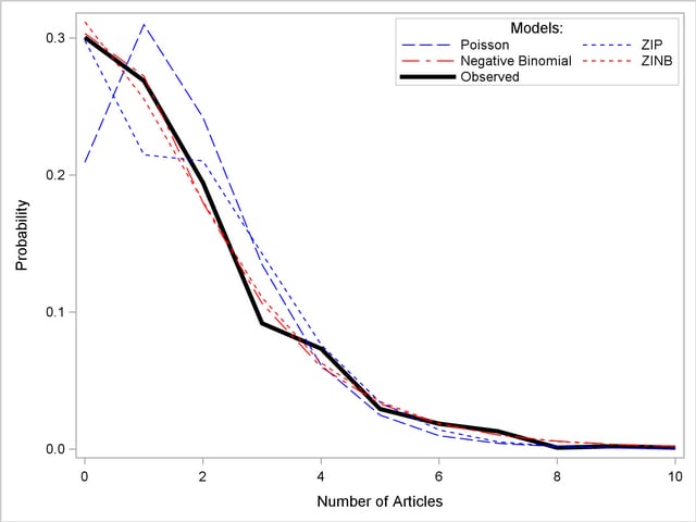
The proportion of zeros predicted by the ZIP model is 0.2986, which is much closer to the observed proportion than the Poisson model. But Output 10.2.4 shows that both models deviate from the observed proportions at one, two, and three articles.
The ZINB model is specified by the DIST=ZINB option. All variables are again used to model both the number of articles and . The METHOD=QN option specifies that the quasi-Newton method be used to fit the model rather than the default Newton-Raphson method. These options are implemented in the following program.
    proc countreg data=long97data;
       model art=fem mar kid5 phd ment / dist=zinb method=qn;
       zeromodel art ~ fem mar kid5 phd ment;
       ods output ParameterEstimates=pe;
    run;

    %probcounts(data=predzip,
                inmodel=pe,
                counts=0 to 10,
                prefix=zinb, out=predzinb)
The estimated parameters of the ZINB model are shown in Output 10.2.3. The test for overdispersion again indicates a preference for the negative binomial version of the zero-inflated model (). The ZINB model also does a good job of estimating the proportion of zeros (0.3119), and it follows the observed proportions well, though possibly not as well as the negative binomial model.
| Model Fit Summary | |
|---|---|
| Dependent Variable | art |
| Number of Observations | 915 |
| Data Set | WORK.LONG97DATA |
| Model | ZINB |
| ZI Link Function | Logistic |
| Log Likelihood | -1550 |
| Maximum Absolute Gradient | 0.00263 |
| Number of Iterations | 81 |
| Optimization Method | Quasi-Newton |
| AIC | 3126 |
| SBC | 3189 |
| Parameter Estimates | |||||
|---|---|---|---|---|---|
| Parameter | DF | Estimate | Standard Error | t Value | Approx Pr > |t| |
| Intercept | 1 | 0.416747 | 0.143596 | 2.90 | 0.0037 |
| fem | 1 | -0.195507 | 0.075592 | -2.59 | 0.0097 |
| mar | 1 | 0.097582 | 0.084452 | 1.16 | 0.2479 |
| kid5 | 1 | -0.151732 | 0.054206 | -2.80 | 0.0051 |
| phd | 1 | -0.000700 | 0.036270 | -0.02 | 0.9846 |
| ment | 1 | 0.024786 | 0.003493 | 7.10 | <.0001 |
| Inf_Intercept | 1 | -0.191684 | 1.322807 | -0.14 | 0.8848 |
| Inf_fem | 1 | 0.635928 | 0.848911 | 0.75 | 0.4538 |
| Inf_mar | 1 | -1.499470 | 0.938661 | -1.60 | 0.1102 |
| Inf_kid5 | 1 | 0.628427 | 0.442780 | 1.42 | 0.1558 |
| Inf_phd | 1 | -0.037715 | 0.308005 | -0.12 | 0.9025 |
| Inf_ment | 1 | -0.882291 | 0.316223 | -2.79 | 0.0053 |
| _Alpha | 1 | 0.376681 | 0.051029 | 7.38 | <.0001 |
The following statements compute the average predicted count probability across all scientists for each count 0, 1, , 10. The averages for each model, along with the observed proportions, are then arranged for plotting by PROC SGPLOT.
    proc summary data=predzinb;
       var poi0-poi10 nb0-nb10 zip0-zip10 zinb0-zinb10;
       output out=mnpoi  mean(poi0-poi10)  =mn0-mn10;
       output out=mnnb   mean(nb0-nb10)    =mn0-mn10;
       output out=mnzip  mean(zip0-zip10)  =mn0-mn10;
       output out=mnzinb mean(zinb0-zinb10)=mn0-mn10;
    run;

    data means;
       set mnpoi mnnb mnzip mnzinb;
       drop _type_ _freq_;
    run;

    proc transpose data=means out=tmeans;
    run;

    data allpred;
       merge obs(where=(art<=10)) tmeans;
       obs=percent/100;
    run;

    proc sgplot;
       yaxis label='Probability';
       xaxis label='Number of Articles';
       series y=obs  x=art / name='obs' legendlabel='Observed'
          lineattrs=(color=black thickness=4px);
       series y=col1 x=art / name='poi' legendlabel='Poisson'
          lineattrs=(color=blue);
       series y=col2 x=art/ name='nb' legendlabel='Negative Binomial'
          lineattrs=(color=red);
       series y=col3 x=art/ name='zip' legendlabel='ZIP'
          lineattrs=(color=blue pattern=2);
       series y=col4 x=art/ name='zinb' legendlabel='ZINB'
          lineattrs=(color=red pattern=2);
       discretelegend 'poi' 'zip' 'nb' 'zinb' 'obs' / title='Models:'
          location=inside position=ne across=2 down=3;
    run;
For each of the four fitted models, Output 10.2.4 shows the average predicted count probability for each article count across all scientists. The Poisson model clearly underestimates the proportion of zero articles published, while the other three models are quite accurate at zero. All of the models do well at the larger numbers of articles.
Copyright © 2008 by SAS Institute Inc., Cary, NC, USA. All rights reserved.