Usage Note 56476: Confidence interval for a ratio of two linear combinations of model parameters
 |  |  |
The following discusses estimation of a ratio of functions of model parameters. Procedures to estimate other ratios such as risk (prevalence) ratios, odds ratios, hazard ratios, and ratios of means are mentioned in the list of Frequently-Asked for Statistics (SAS Note 30333).
Two methods for estimating the confidence limits for a ratio are discussed using the common example of estimation of the ED50 and the relative potency. In bioassay studies that investigate the effect of various doses of one or more drugs, the ED50 is the effective dose at which 50% of the subjects respond. The relative potency is the ratio of doses of two drugs that produce the same response. Both the ED50 and the relative potency are estimated as ratios of model parameters in a binary response model.
Quantal Bioassay Example
Stokes et. al. (2000) discuss a study on mice comparing two drugs applied at several doses. The data are presented below. The response (death) probability, p, is calculated as the ratio of the number of deaths, NDEAD, to the number of mice, TOTAL. The dose at which a 50% response is observed in each dose is recorded in variable REF. The log of dose and REF are also computed:
      data assay;
         input drug $ dose ndead total;
         p=ndead/total;
         if p=0.5 then ref=dose;
         ldose=log(dose);
         ldref=log(ref);
         datalines;
      N   0.01 0 30
      N   0.03 1 30
      N   0.10 1 10
      N   0.30 1 10
      N   1.00 4 10
      N   3.00 4 10
      N  10.00 5 10
      N  30.00 7 10
      S   0.30 0 10
      S   1.00 0 10
      S   3.00 1 10
      S  10.00 4 10
      S  30.00 5 10
      S 100.00 8 10
      ;
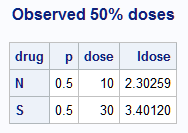
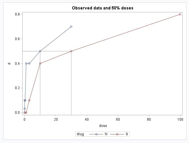
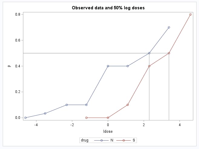
The following statements plot the observed response probabilities against both the dose and log(dose). Because in each drug there happens to be a dose at which 50% of mice respond, it is also possible to highlight the dose and log(dose) values at which a 50% response is observed. These data points are displayed by PROC PRINT. Of course, this is not generally true in observed data. An estimate of the N:S relative potency using the observed raw data is 10/30 = 0.33:
     proc print data=assay;
        where p=0.5;
        id drug;
        var p dose ldose;
        title "Observed 50% doses";
        run;
     proc sgplot;
        series y=p x=dose / markers group=drug;
        dropline y=0.5 x=ref / dropto=both;
        title "Observed data and 50% doses";
        run;
     proc sgplot;
        series y=p x=ldose / markers group=drug;
        dropline y=0.5 x=ldref / dropto=both;
        title "Observed data and 50% log doses";
        run;
   |
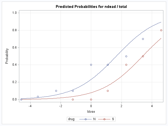
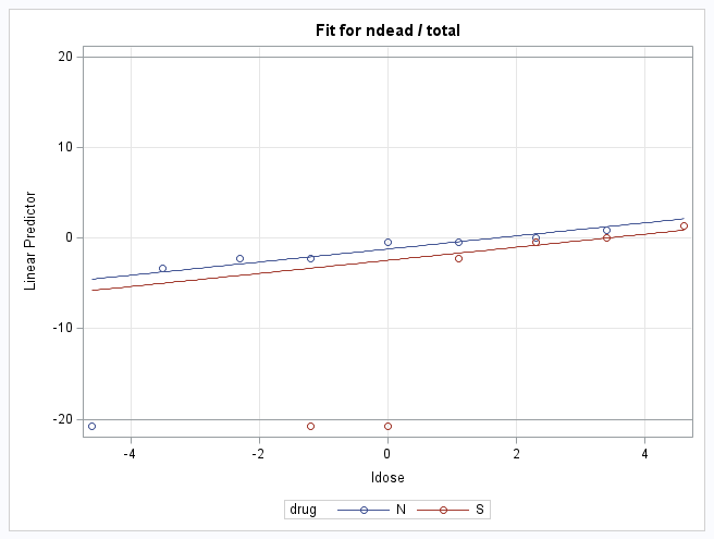
A sequence of logistic models fit to the data (not shown) suggests that a model with separate intercepts for the drugs but with a common slope fits well. The following statements fit this final model. Note that with the NOINT option, the two DRUG parameters are the intercepts for the two drugs. See SAS Note 24177 for more information about assessing the need for separate slopes when modeling data from multiple groups. The OUTEST= and COVOUT options are not needed to fit the model but provide a data set that contains the estimated model parameters and covariance matrix for use later. The STORE statement is used to save the model information for use later by the NLEST macro. The EFFECTPLOT statements show the fitted model on both the probability scale and the logit (linear predictor) scale:
      proc logistic data=assay outest=parms covout;
         class drug / param=glm;
         model ndead/total = drug ldose / noint;
         effectplot slicefit(sliceby=drug);
         effectplot slicefit(sliceby=drug) / link;
         store out=assaymod;
         run;
In the plots, the points on the LDOSE axis where a line at p=0.5 or logit=0 cross the fitted group lines are the estimated log(dose) values producing 50% response under the model. Note that the logit=0 when p=0.5. In the first plot against the response probability, notice that the log(dose) value producing 50% response is approximately equal to the observed value for the S drug but is a bit lower than observed for the N drug.
  |
|||||||||||||||||||||||||||||||||||
To estimate the ED50 for each drug (the dose producing a 50% response) as well as their relative potency (the ratio of those doses) under the model, Stokes et al. (2000) show that the estimates of the ED50 for drug N and drug S are -aN/b and -aS/b, where aN and aS are the estimated intercepts for drugs N and S, and b is the estimated log dose (LDOSE) parameter, the common slope. Since each estimate is of the log dose, the difference of the estimates is the log relative potency. As shown by Stokes et al., the estimate of the relative potency (N:S) therefore is exp[(aS - aN)/b]. Notice that all these statistics are ratios of functions of the model parameters.
There are two methods for obtaining the confidence limits for a ratio of linear combinations of model parameters—the method using Fieller's theorem and the delta method. Zerbe (1978) shows how confidence limits based on Fieller's theorem can be obtained for any ratio of linear combinations of model parameters in a generalized linear model. The delta method is a general method that provides an approximate estimate of the variance of nonlinear functions of random variables. Hirschberg and Lye (2010) compare the two methods and discuss when they produce similar results.
Note that for the particular case of estimating the effective dose for some response rate (ED50 or other response rate), the INVERSECL option in the MODEL statement of PROC PROBIT can be used to obtain confidence limits based on Fieller's theorem.Note1 The methods discussed below can be used more generally to estimate ratios.
Delta Method Using the NLEST Macro
Since the ED50 and relative potency are nonlinear functions of model parameters, they can be estimated using the NLEST macro (SAS Note 58775). The NLEST macro uses the fitted model information saved by the STORE statement in PROC LOGISTIC. It then uses PROC NLMIXED to estimate the functions. The delta method is used to obtain confidence limits. By default, 95% large sample confidence intervals are given. When estimating a single function, specify the function in f= and a suitable label in label= in the macro. When estimating several functions, they can be specified in a data set with appropriate labels. The following statements estimate the ED50 of log dose and dose for the two drugs as well as the log relative potency and relative potency by specifying appropriate functions of the model parameters in data set FD and specifying that data set in fdata= in the macro call. Since the relative potency is a ratio of the dose estimates, it is of interest to test the null hypothesis that it equals 1 rather than 0. This is done in a separate call of the NLEST macro by specifying null=1. When null= is not specified, the macro tests the null hypothesis of equality to zero. The model parameters in the estimating functions are referred to using names of the form B_P1, B_P2, and so on in the order as presented by PROC LOGISTIC. See the description of the NLEST macro for details about displaying parameter names and using the macro:
      data fd;
        length label f $32767;
        infile datalines delimiter=',';
        input label f;
        datalines;
      Drug S log ED50,-b_p2/b_p3
      Drug N log ED50,-b_p1/b_p3
      N:S log(Rel. Potency),(b_p2-b_p1)/b_p3
      Drug S ED50,exp(-b_p2/b_p3)
      Drug N ED50,exp(-b_p1/b_p3)
      ;
      %nlest(instore=assaymod, fdata=fd)
      %nlest(instore=assaymod, label=N:S Rel. Potency, f=exp((b_p2-b_p1)/b_p3), null=1)
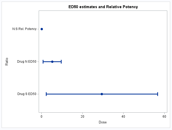
The estimates and confidence intervals for all ratios appear in the Estimate, Lower, and Upper columns of the Nonlinear Function Estimate tables. For example, the estimated log dose of Drug S that produces a 50% response is 3.3835 with 95% confidence interval (2.4559, 4.3110). The estimates and confidence intervals for both drugs on the dose scale are also provided and are 29.47 for drug S and 5.2 for drug N. As can be seen in the raw data and in plots from the EFFECTPLOT statements, the model estimate for drug S is close to the observed value in the data, but the drug N estimate is a bit lower.
The N:S log relative potency estimate is -1.7341 with 95% confidence interval (-2.9536, -0.5146). The estimated N:S relative potency is 0.1766 and differs significantly from 1 (p<0.0001). The 95% confidence interval for the relative potency is (-0.0388, 0.3919). Compare this to the relative potency, 0.33, seen in the raw data. Note that the 95% confidence interval includes estimates observed in the raw data:
  |
Delta Method Using PROC NLMIXED
Estimation by the delta method can also be done by fitting the model in PROC NLMIXED and specifying the ratio in the ESTIMATE statement. The following statements fit the same logistic model as above in PROC NLMIXED. The first three ESTIMATE statements estimate the log ED50 for each drug and the log relative potency. The estimates on the dose scale are provided next. The final ESTIMATE statement subtracts 1 from the relative potency estimate to test that the relative potency equals 1. The delta method is used by the ESTIMATE statements to approximate the variance of each ratio and provide the confidence limits. The ODS OUTPUT statement saves the results of the ESTIMATE statements in a data set named DELTA. The DF=1E8 option is specified in order to provide large-sample confidence intervals:
      proc nlmixed data=assay df=1e8;
         p=logistic(bdrugs*(drug="S") + bdrugn*(drug="N") + bdose*ldose);
         model ndead ~ binomial(total,p);
         estimate "Drug S log ED50" -bdrugs/bdose;
         estimate "Drug N log ED50" -bdrugn/bdose;
         estimate "N:S log(Rel. Potency)" (bdrugs-bdrugn)/bdose;
         estimate "Drug S ED50" exp(-bdrugs/bdose);
         estimate "Drug N ED50" exp(-bdrugn/bdose);
         estimate "N:S Rel. Potency" exp((bdrugs-bdrugn)/bdose);
         estimate "Test Rel.Pot.=1" exp((bdrugs-bdrugn)/bdose)-1;
         ods output AdditionalEstimates=delta;
         run;
The results are the same as from the NLEST macro above.
Fieller's Method Using SAS/IML®
Stokes et. al. (2000) present a SAS/IML module based on Zerbe (1978) that implements Fieller's method.Note2 The following statements create a macro using similar code. This code must be run in order to define the Fieller macro and make it available for use:
    %macro Fieller(data=, out=RatioCI, num=, den=, label=Ratio, alpha=.05, intercept=yes);
      data _inest;
        set &data;
        drop _LNLIKE_
          %if %substr(%upcase(&intercept),1,1)=N %then Intercept;
        ;
        run;
      proc iml;
        use _inest;
        read all var _num_ into beta where (_type_="PARMS");
        beta=beta`;
        read all var _num_ into cov where (_type_="COV");
        k={ &num }; h={ &den };
        ratio=(k*beta) / (h*beta);
        tsq=probit(1-&alpha/2)**2;
        a=(h*beta)**2-(tsq)*(h*cov*h`);
        b=2*(tsq*(k*cov*h`)-(k*beta)*(h*beta));
        c=(k*beta)**2 -(tsq)*(k*cov*k`);
        disc=((b**2)-4*a*c);
        if (disc<=0 | a<=0) then do;
          print "ERROR: confidence interval can't be computed";
          stop;
        end;
        sroot=sqrt(disc);
        l_b=((-b)-sroot)/(2*a);
        u_b=((-b)+sroot)/(2*a);
        estlims=ratio||l_b||u_b;
        lname={"Estimate", "LCL", "UCL"};
        create &out from estlims[colname=lname];
        append from estlims;
        quit;
      data &out;
        set &out;
        Ratio="&label";
        run;
      proc print data=&out;
        id Ratio;
        run;
    %mend;
The following statements call the macro three times to estimate the ED50 for each drug and the log relative potency. The macro cannot be used with this model to estimate the ED50 or relative potency on the dose scale. The data set created by the OUTEST= and COVOUT options in PROC LOGISTIC should be specified in DATA=. OUT= names the data set that contains the estimates and confidence intervals. If omitted, the data set name is RatioCI. NUM= and DEN= specify vectors of coefficients, which when multiplied by the vector of model parameters produce the linear combinations that define the numerator and denominator of the ratio of interest. For example, in the first macro call below, the NUM= vector (-1 0 0) multiplies the parameter vector (aN aS b) yielding -aN, and the DEN= vector (0 0 1) yields b, the numerator and denominator of the Drug N ED50, -aN/b. INTERCEPT= specifies whether an overall intercept was included in the model. In this case, the overall intercept was omitted by the NOINT option, so INTERCEPT=NO. Omit OPTION= when the overall intercept is included in the model. LABEL= provides a label for the ratio in the displayed results. By default, the macro produces a 95% confidence interval corresponding to an alpha level of 0.05. The confidence level can be changed by specifying ALPHA= in the macro:
      %Fieller(data=parms, out=DN, num=-1 0 0, den=0 0 1, label=Drug N log ED50, intercept=no)
      %Fieller(data=parms, out=DS, num=0 -1 0, den=0 0 1, label=Drug S log ED50, intercept=no)
      %Fieller(data=parms, out=RP, num=-1 1 0, den=0 0 1, label=N:S log(Rel. Potency), intercept=no)
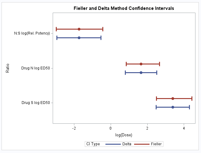
Notice that the confidence limits using Fieller's method are slightly different from those produced above by the delta method:
   |
Hirschberg and Lye (2010) discuss conditions under which the delta method and Fieller's theorem produce similar confidence intervals. They note:
"As a general rule, when the sign of the estimated ratio is the same as the sign of the estimated correlation between the numerator and denominator, one can consider the Delta interval and thus avoid the computational burden involved in using the Fieller interval. However, when these signs differ and the precision of the denominator is low, the Fieller interval should be used."
They conclude that:
"... when the Fieller and Delta intervals differ, the Fieller interval results in better coverage, and in some cases, this advantage can be very large."
In this case, the estimated ratios are all positive and the correlation between numerator and denominator is also positive for each ratio, suggesting that either method should be reasonable.
The following statements produce a plot that compares the Fieller and delta method intervals:
      data delta2;
        set delta (where=(label ? "log"));
        Ratio=label; LCL=Lower; UCL=Upper; type="Delta  ";
        keep Ratio Estimate LCL UCL type;
        run;

      data fieller;
        length Ratio $ 25;
        type="Fieller";
        set DN DS RP;
        run;

      data RatioCIs;
        length Ratio $ 25;
        set delta2 fieller;
        run;

      proc sgplot data=RatioCIs;
        highlow y=ratio low=lcl high=ucl /
                group=type groupdisplay=cluster clusterwidth=0.5
                highcap=serif lowcap=serif lineattrs=(thickness=3);
        scatter y=ratio x=estimate / group=type groupdisplay=cluster
                clusterwidth=0.5 markerattrs=(symbol=circlefilled size=10);
        xaxis label="log(Dose)";
        label type="CI Type";
        title "Fieller and Delta Method Confidence Intervals";
        run;
As can be seen in the plot, the intervals are quite similar for each ratio. Note that the Fieller intervals are not necessarily symmetric about the ratio estimate:
 |
These statements plot the ED50 estimates on the dose scale as well as the estimate of the relative potency along with their 95% confidence intervals:
      data dscale;
        set delta;
        if _N_ in (4,5,6);
        Ratio=label; LCL=Lower; UCL=Upper;
        keep Ratio Estimate LCL UCL;
        run;
      proc sgplot data=dscale noautolegend;
        highlow y=ratio low=lcl high=ucl /
                highcap=serif lowcap=serif lineattrs=(thickness=3);
        scatter y=ratio x=estimate / markerattrs=(symbol=circlefilled size=10);
        xaxis label="Dose";
        title "ED50 estimates and Relative Potency";
        run;
 |
__________
Note 1: PROC PROBIT can fit probit or logistic models. The INVERSECL option estimates the effective dose for the drug that is treated as the reference level. By default, the INVERSECL option provides effective dose estimates for a range of response rates. You can specify one or more specific rates with the PROB= suboption. The following statements fit the same logistic model as above and estimate the ED50 for each drug using Fieller's method:
      proc probit data=assay log;
        class drug(ref="N");
        model ndead/total = drug dose / inversecl(prob=.5) d=logistic;
        run;
      proc probit data=assay log;
        class drug(ref="S");
        model ndead/total = drug dose / inversecl(prob=.5) d=logistic;
        run;
Note 2: In the interval computations, Zerbe (1978) uses a quantile from the t distribution with n-p degrees of freedom, where n is the sample size and p is the number of model parameters. This macro uses a quantile from the standard normal distribution, which should produce similar results in large samples when n is much larger than p.
References
Hirschberg, J. and Lye, J. (2010), "A Geometric Comparison of the Delta and Fieller Confidence Intervals," The American Statistician, 64:3, 234-241.
Stokes, M.E., Davis, C.S., and Koch G.G. (2000), Categorical Data Analysis Using SAS®, Third Edition, Cary, NC: SAS Institute Inc.
Zerbe, G.O. (1978), "On Fieller's Theorem and the General Linear Model", The American Statistician, 32:3, 103-105.
Operating System and Release Information
| Product Family | Product | System | SAS Release | |
| Reported | Fixed* | |||
| SAS System | SAS/STAT | z/OS | ||
| Z64 | ||||
| OpenVMS VAX | ||||
| Microsoft® Windows® for 64-Bit Itanium-based Systems | ||||
| Microsoft Windows Server 2003 Datacenter 64-bit Edition | ||||
| Microsoft Windows Server 2003 Enterprise 64-bit Edition | ||||
| Microsoft Windows XP 64-bit Edition | ||||
| Microsoft® Windows® for x64 | ||||
| OS/2 | ||||
| Microsoft Windows 8 Enterprise 32-bit | ||||
| Microsoft Windows 8 Enterprise x64 | ||||
| Microsoft Windows 8 Pro 32-bit | ||||
| Microsoft Windows 8 Pro x64 | ||||
| Microsoft Windows 8.1 Enterprise 32-bit | ||||
| Microsoft Windows 8.1 Enterprise x64 | ||||
| Microsoft Windows 8.1 Pro | ||||
| Microsoft Windows 8.1 Pro 32-bit | ||||
| Microsoft Windows 95/98 | ||||
| Microsoft Windows 2000 Advanced Server | ||||
| Microsoft Windows 2000 Datacenter Server | ||||
| Microsoft Windows 2000 Server | ||||
| Microsoft Windows 2000 Professional | ||||
| Microsoft Windows NT Workstation | ||||
| Microsoft Windows Server 2003 Datacenter Edition | ||||
| Microsoft Windows Server 2003 Enterprise Edition | ||||
| Microsoft Windows Server 2003 Standard Edition | ||||
| Microsoft Windows Server 2003 for x64 | ||||
| Microsoft Windows Server 2008 | ||||
| Microsoft Windows Server 2008 R2 | ||||
| Microsoft Windows Server 2008 for x64 | ||||
| Microsoft Windows Server 2012 Datacenter | ||||
| Microsoft Windows Server 2012 R2 Datacenter | ||||
| Microsoft Windows Server 2012 R2 Std | ||||
| Microsoft Windows Server 2012 Std | ||||
| Microsoft Windows XP Professional | ||||
| Windows 7 Enterprise 32 bit | ||||
| Windows 7 Enterprise x64 | ||||
| Windows 7 Home Premium 32 bit | ||||
| Windows 7 Home Premium x64 | ||||
| Windows 7 Professional 32 bit | ||||
| Windows 7 Professional x64 | ||||
| Windows 7 Ultimate 32 bit | ||||
| Windows 7 Ultimate x64 | ||||
| Windows Millennium Edition (Me) | ||||
| Windows Vista | ||||
| Windows Vista for x64 | ||||
| 64-bit Enabled AIX | ||||
| 64-bit Enabled HP-UX | ||||
| 64-bit Enabled Solaris | ||||
| ABI+ for Intel Architecture | ||||
| AIX | ||||
| HP-UX | ||||
| HP-UX IPF | ||||
| IRIX | ||||
| Linux | ||||
| Linux for x64 | ||||
| Linux on Itanium | ||||
| OpenVMS Alpha | ||||
| OpenVMS on HP Integrity | ||||
| Solaris | ||||
| Solaris for x64 | ||||
| Tru64 UNIX | ||||
| Type: | Usage Note |
| Priority: | |
| Topic: | Analytics ==> Analysis of Variance Analytics ==> Categorical Data Analysis Analytics ==> Regression SAS Reference ==> Procedures ==> LOGISTIC SAS Reference ==> Procedures ==> IML SAS Reference ==> Procedures ==> NLMIXED SAS Reference ==> Macro |
| Date Modified: | 2024-10-24 09:38:43 |
| Date Created: | 2015-08-21 16:20:18 |