Usage Note 23003: Estimating a relative risk (also called risk ratio, prevalence ratio)
 |  |  |
The relative risk (also known as the risk ratio or prevalence ratio) is the ratio of event probabilities at two levels of a variable or two settings of the predictors in a model, where the "event" is the response level of interest. The relative risk can be estimated in the context of a model or using a nonmodeling approach. The estimation of model parameters can be avoided by using PROC FREQ even when more than one predictor is involved.
When assessing the effect of a particular predictor in a model, it is of interest to estimate the relative risk for that predictor adjusted for the effects of the other predictors. For a continuous predictor, the relative risk, px+1/px, is interpreted as the change in event probability for a unit increase in the predictor. For a categorical predictor, the relative risk, pxi /pxj , is interpreted as the change in event probability when changing from level j of the predictor to level i.
When the variable whose relative risk is to be estimated is involved in interaction in a model, the relative risk changes depending on the level of the interacting variable(s). When the interacting variable is continuous, the relative risk can be estimated at various levels of the interacting variable and plotted as a function of the interacting variable as discussed in SAS Note 69621.
When prevalence of the event is low, the odds ratio provides a good estimate of the relative risk (Agresti 2002). In this situation, the odds ratio estimates from PROC FREQ or the usual logistic model (the default logit-linked, binomial model) fit by PROC LOGISTIC can be used to estimate relative risks. If the event probability is not small, then other approaches can be used. Four methods are presented below – estimation without a model, estimation using a macro to evaluate the relevant nonlinear combination of logistic model parameters, estimation using a log-linked binomial model, and using a Poisson approach with GEE estimation (Zou, 2004). Estimation of relative risks from multinomial response models is discussed and illustrated in SAS Note 57798.
Nonmodeling Approach Using PROC FREQ
In the simplest case of a single binary predictor of a binary response, the data can be arranged as a 2x2 table and the relative risk is estimated using the RELRISK option in the TABLES statement of PROC FREQ. For example, suppose a group of 100 men and an independent group of 100 women are asked a Yes/No question and 30 men responded Yes while 45 women responded Yes. The data are arranged in a 2x2 table and the relative risk estimate is requested using these statements:
      data question;
        input Gender $ Response $ Count;
        datalines;
      Women Yes 45
      Women  No 55
      Men   Yes 30
      Men    No 70
      ;
      proc freq data=question order=data;
        weight Count;
        tables Gender*Response / relrisk;
        run;
The RELRISK option provides relative risk and odds ratio estimates. Since the level of interest (the event level) is Response=Yes, and since Yes is the first column (because of the data order and the use of the ORDER=DATA option), the relative risk estimate is provided in the "Cohort (Col1 Risk)" row of the "Estimates of the Relative Risk" table. The relative risk of the Yes response for Women relative to Men is 1.50 with confidence interval (1.0365, 2.1707). Note that the odds ratio estimate of 1.91 and that the event probability is not small – approximately 37.5% overall.
|
|||||||||||||||||||||||||||||||||||||||||||||||||||||||||||||||||||||||||||||||||
If there are multiple predictors, the relative risk for a particular predictor can be obtained from the CMH option with the other predictors specified first in the table definition. Variables preceding the final two variables (which specify the row and column variables of the table) are treated as stratification variables. An example of this is given below in the section describing the modified Poisson approach.
Note that PROC FREQ can be used to estimate the relative risk only when the row variable has two levels.
Nonlinear Estimate Using a Logistic Model
Since the log odds (also called the logit) is the response function in a logistic model, such models enable you to estimate the log odds for populations in the data. A population is a setting of the model predictors. By exponentiating, you can estimate the odds. Similarly, the difference between two populations results in an estimated difference in log odds that is equivalent to a log odds ratio. Again, by exponentiating, you can estimate the odds ratio comparing the populations. So, simple linear combinations of logistic model parameters can be used to obtain estimates of odds and odds ratios.
However, the ratio of event probabilities (population means) cannot be obtained in this way. To estimate the relative risk (a ratio of probabilities), you need to estimate a nonlinear function of the parameters of the logistic model. While the ESTIMATE statement in PROC LOGISTIC only estimates linear combinations of model parameters, the NLEstimate macro (SAS Note 58775) can estimate any linear or nonlinear combinations that you specify. Similarly, PROC NLMIXED and its ESTIMATE statement can be used to fit the model and estimate nonlinear combinations. The NLMeans macro simplifies the task of estimating and testing differences, ratios, or contrasts of means.
For the above example, the logistic model can be written as follows:
p = [1 + e-(β0 + β1I(Women))]-1 ,
where I(Women)=1 if GENDER="Women", and 0 otherwise. The same model can be written in terms of the log odds (logit) as follows:
logit(p) = β0 + β1I(Women)
and can be fit using PROC LOGISTIC as shown in the following statements. The LSMEANS statement provides estimates of the log odds for each gender. The ILINK option adds estimates of the event probabilities by applying the inverse of the logit link. The E option produces a table of coefficients of the linear combination of parameters that define the log odds for each gender. The table is saved by the ODS OUTPUT statement for use later with the NLMeans macro. The STORE statement saves the fitted model for use with the NLMeans and NLEstimate macros:
      proc logistic data=question;
        freq count;
        class gender(ref="Men") / param=glm;
        model response(event="Yes")=gender;
        lsmeans gender / e ilink;
        ods output coef=coeffs;
        store out=ques;
        run;
These partial results show the parameters of the fitted logistic model followed by the estimated gender odds ratio that matches the result above from PROC FREQ. Finally, the coefficients defining the log odds and the estimated log odds and event probabilities are shown. Note that the event probabilities, 0.45 and 0.3, match the probabilities shown in the table from PROC FREQ:
|
|||||||||||||||||||||||||||||||||||||||||||||||||||||||||||||||||||||||||||||||||||||||||||||||
Using the NLMeans Macro
The relative risk can be most easily estimated using the NLMeans macro as a ratio of the event probabilities. To use the macro, you provide the saved model from the STORE statement, the saved table of coefficients from the LSMEANS / E statement, and the link function used in the model. By default, the NLMeans macro estimates and tests pairwise differences among the mean estimates. In this example, that would be the difference in gender event probabilities. To request that the ratio be estimated rather than the difference, specify options=ratio. By default, the null hypothesis tested by the macro is a test of equality to zero. For the relative risk, the null hypothesis of interest is a test that the relative risk equals one. To do that, specify null=1 (requires version 1.3 or later of the NLMeans macro and version 1.8 or later of the NLEST macro):
      %nlmeans(instore=ques, coef=coeffs, link=logit, options=ratio,
               null=1, title=Relative Risk)
The Label indicates that the first mean (Women) is divided by the second mean (Men). If the reciprocal of this is desired, add the reverse option: options=ratio reverse. The estimated relative risk is 1.5 with 95% large-sample confidence interval (0.95, 2.05) and differs significantly from 1 (p=0.0771). Notice that the estimated relative risk and its confidence interval are quite similar to the estimate produced by PROC FREQ above. Results differ slightly due to the different estimation methods used:
|
Using the NLEST/NLEstimate Macro
The NLEST/NLEstimate macro also uses the fitted model saved by the STORE statement in PROC LOGISTIC. It then uses PROC NLMIXED to estimate the specified function of model parameters. The delta method is used to obtain confidence limits. You write the function to be estimated using the parameter names and specify it in the f= macro parameter. A label can be provided in the label= parameter. See the description of the NLEST macro for details about displaying parameter names and using the macro. The function LOGISTIC(x) = [1 + e-(x)]-1 makes it easy to write the relative risk as a ratio of probabilities. As discussed above, to test that the relative risk equals 1, specify null=1 (requires version 1.8 or later of the NLEST macro):
      %nlest(instore=ques, label=Rel. Risk (Women/Men),
             null=1, f=logistic(b_p1+b_p2)/logistic(b_p1))
The results match those from the NLMeans macro above:
|
Using PROC NLMIXED
PROC NLMIXED does not have a FREQ statement for aggregated data like the data above. One way to handle this is to expand the aggregated data into single-subject data as done in the following DATA step. If the data were already in single-subject form, no preprocessing step would be needed. A binary response variable, Y, is created with values 1 (for the event) and 0. This is the response that is modeled in PROC NLMIXED:
      data q2;
       set question;
       y=(response="Yes");
       do i=1 to count;
        output;
       end;
       run;
In PROC NLMIXED, you write the model on the event probability, p, and then specify p in the BINARY distribution option in the MODEL statement. The LOGISTIC function is again used, this time to specify the logistic model and then again in the ESTIMATE statements to define the ratio of probabilities for women and men. The first ESTIMATE statement provides an estimate and confidence interval for the relative risk as well as a test that the relative risk equals zero. To test that the relative risk equals 1 rather than 0, the second ESTIMATE statement subtracts 1 from the function:
      proc nlmixed data=q2;
        p=logistic(b0 + b1*(gender="Women"));
        model y ~ binary(p);
        estimate "Rel. Risk (Women/Men)" logistic(b0+b1) / logistic(b0);
        estimate "Test Rel. Risk = 1" (logistic(b0+b1) / logistic(b0))-1;
        run;
The results are similar to those from the NLEST/NLEstimate macro above:
Log-linked Binomial Model
As shown below, exponentiating a parameter estimate in a log-linked binomial model directly estimates the relative risk. Here is the one-variable, linear log-linked model:
| log(p) = a + bx |
Under this model, a one-unit increase in the predictor yields the following results:
| log(p1) = a + b(x+1) = a + bx + b | (1) |
and
| log(p2) = a + bx | (2) |
Subtracting (2) from (1):
| log(p1) - log(p2) = b |
But note that log(p1) - log(p2) = log(p1/p2) = log(relative risk), implying that the parameter estimate for the predictor, b, estimates the log relative risk. So, exponentiating the parameter estimate, eb, provides an estimate of the relative risk.
You can fit the log-linked binomial model by using PROC GENMOD with the DIST=BINOMIAL and LINK=LOG options. However, using the log link can result in fitting problems (SAS Note 23001) because the log does not ensure that predicted probabilities are mapped to the [0,1] range that is required for probabilities. Deddens, Petersen, and Lei (2003) suggest routinely using the MODEL statement option INTERCEPT=-4 when fitting this model. This option provides a starting value of -4 for the intercept in the maximum likelihood estimation process. The sense of doing this can be seen by noting that 0 < p < 1, which implies that log(p) < 0. When all predictors are zero or at their reference levels, the intercept estimates log(p), so it makes sense to start its estimation in the negative range.
Deddens, et. al. note that PROC GENMOD still might fail to fit the log-linked model because the solution falls on the boundary of the parameter space. When this happens, they suggest that the solution can often be found by fitting the model to a data set consisting of many copies of the original data augmented with one copy in which the response values are opposite those in the original data. This puts the solution in the parameter space where the optimization algorithm can find it. While this provides good estimates of the model parameters, and therefore good estimates of the adjusted relative risks, the standard errors are reduced due to the replication of the data. To correct this, they multiply the standard errors by the square root of the number of copies and recompute tests and confidence intervals. The same effect might be achieved by using weights normalized to the actual sample size so that replication of the data and adjustment of the standard errors are unnecessary.
Based on the example presented by the authors, the following statements fit the log-linked model to the original data augmented with a copy of the data having reversed responses. So that relative risk computation can be illustrated for both continuous and categorical predictors, a categorical variable, A, is introduced. The authors' original observations are in the A=1 level. Data are provided for an additional level, A=2. The actual values are assigned a weight of 10,000 and the reversed-response observations are assigned a weight of 1. To normalize the weights so that they sum to the original sample size, the weights are multiplied by the true sample size, 20, and divided by the sum of the weights, 200,020. The sum of the normalized weights is the actual sample size, 20. This adjusts the standard errors and related statistics so that they are correct.
In the PROC GENMOD statements below, the LSMEANS statement estimates the individual risks and relative risk comparing level A=2 to level A=1 at the mean of X. The EXP option adds the Exponentiated columns in the Least Squares Means table showing the estimated risk, standard error, and confidence interval in each level of A. It also adds the Exponentiated columns in the Differences table showing the estimated relative risk and its confidence interval. The ESTIMATE statement provides the relative risk estimate for a one unit increase in X in the authors' original data in A=1. The log relative risk estimate appears in the "L'Beta Estimate" column, and the relative risk estimate in the "Mean Estimate" column of the "Contrast Estimate Results" table NOTE.
     data a;
         do a=1,2;
         do x=1 to 10;
            /* read the actual data, set weights to 10000, then normalize */
            input y @@; f=10000 * 20/200020; output;
            /* create reverse-response data, set weights to 1, then normalize */
            y=1-y;      f=    1 * 20/200020; output;
         end; end;
         datalines;
     0 0 0 0 1 0 1 1 1 1
     0 1 0 1 0 0 0 1 1 1
     ;

     proc genmod data=a;
         class a;
         model y(event="1") = x|a / dist=binomial link=log;
         weight f;
         lsmeans a / diff exp cl;
         estimate "RR (X+1)/X" x 1 x*a 1;
         run;
The results from the ESTIMATE statement provide the estimate and confidence interval for both the relative risk ("Mean Estimate") and the log relative risk ( "L'Beta Estimate") in A=1. The results indicate that the event (Y=1) is 1.23 times more likely when the predictor, X, increases by one unit. The estimated risks in each level of A appear in the Exponentiated column in the Least Squares Means table. The risk estimate in A=1 is 0.3898 and in A=2 is 0.4533. The risk ratio estimate, 0.8601, appears in the Exponentiated column in the Differences table along with its confidence interval (0.2707, 2.7327):
|
|||||||||||||||||||||||||||||||||||||||||||||||||||||||||||||||||||||||||||||||||||||||||||||||||||||||||||||||||||||
Zou's Modified Poisson Approach
Zou shows that when a Poisson model is fit to the binary response, the robust variance estimator provided by the REPEATED statement in PROC GENMOD gives a proper estimate of the standard error of the relative risk. Note that the REPEATED statement implements the Generalized Estimating Equations (GEE) estimation method which is typically used for repeated measures or longitudinal data. However, the method can also be used for data without repeated measurements when a robust estimate of variance is needed.
The following statements create the data set for the 28-day mortality study shown in Zou (2004) and fit the modified Poisson model. Dr. Zou kindly provided the code (modified to use the LSMEANS statement):
      data example2;
        input strata treat outcome count;
        do i=1 to count;
          id+1; output;
        end;
        datalines;
      1 1 1 12
      1 1 0 1
      1 0 1 6
      1 0 0 4
      2 1 1 5
      2 1 0 8
      2 0 1 1
      2 0 0 11
      3 1 1 5
      3 1 0 18
      3 0 1 1
      3 0 0 21
      ;

      proc genmod data=example2;
        class id strata treat(ref="0");
        model outcome = treat strata / dist=poisson link=log;
        repeated subject=id;
        lsmeans treat / diff exp cl;
        run;
Since TREAT is a CLASS predictor using the default GLM parameterization, the LSMEANS statement can be used to obtain the log relative risk (Estimate) and relative risk (Exponentiated) estimates. From the results, the estimate of the relative risk is 2.30 with confidence interval (1.27, 4.15):
|
||||||||||||||||||||||||||||||||||||
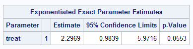
A similar estimate is produced using exact Poisson regression but with somewhat wider confidence interval. Note however that the exact method can require substantial resources (memory and time), particularly with larger data sets, and this can make the exact method infeasible:
       proc genmod data=example2;
         class strata treat(ref="0")/param=ref;
         model outcome = treat strata / dist=poisson;
         exact treat / estimate=both;
         run;
 |
For comparison, Zou fits the log-linked binomial model:
      proc genmod descending data=example2;
        class strata treat(ref="0");
        model outcome = treat strata / dist=binomial link=log;
        lsmeans treat / diff exp cl;
        run;
The estimate from this model is somewhat smaller — 1.94 with confidence interval (1.05, 3.59):
|
||||||||||||||||||||||||||||||||||||
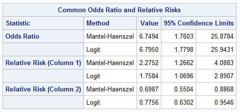
Zou also compares the results to the nonmodeling approach by using the Mantel-Haenszel method available in PROC FREQ. The CMH option is used in order to accommodate the strata. The NOPRINT option is also used to suppress the display of the TREAT*OUTCOME tables for all of the strata. While there are only three stratum-specific tables in this example, in general there could be a large number. Using the NOPRINT option limits the displayed results to the statistical tables produced by the CMH option:
      proc freq data=example2 order=data;
        tables strata*treat*outcome / cmh noprint;
        run;
Since the ORDER=DATA option with these data places the event level in the first column of the table, the Mantel-Haenszel relative risk estimate appears in the "Relative Risk (Column 1)" row as 2.28 with confidence interval (1.27.4.09):
 |
References
Deddens, J.A., Petersen, M.R., and Lei, X. (2003), Estimation of prevalence ratios when PROC GENMOD does not converge, Proceedings of the Twenty-Eighth Annual SAS® Users Group International Conference, Seattle, WA.
Zou, G. (2004), "A Modified Poisson Regression Approach to Prospective Studies with Binary Data," Am. J. Epidemiol., 159:702-706.
_____
NOTE: In releases prior to SAS® 9.2, the EXP option is needed to exponentiate the contrast (in this case, only the parameter for X) resulting in a relative risk estimate for a unit increase in X. Beginning in SAS 9.2, the EXP option is not needed since estimates of the contrast applying the inverse link function (labeled "Mean") are provided by default.
Operating System and Release Information
| Product Family | Product | System | SAS Release | |
| Reported | Fixed* | |||
| SAS System | SAS/STAT | All | n/a | |
| Type: | Usage Note |
| Priority: | low |
| Topic: | SAS Reference ==> Procedures ==> LOGISTIC SAS Reference ==> Procedures ==> GENMOD SAS Reference ==> Procedures ==> FREQ SAS Reference ==> Procedures ==> NLMIXED SAS Reference ==> Macro |
| Date Modified: | 2025-11-13 15:50:33 |
| Date Created: | 2002-12-16 10:56:41 |