Distribution Analysis Task

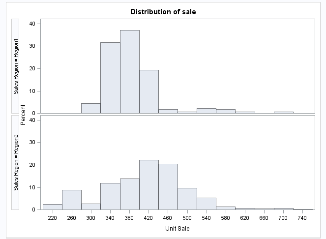
Example: Distribution Analysis of Sales for Each Region

About the Distribution Analysis Task

Distribution analysis provides information about the distribution of numeric variables. A variety of plots such as histograms, probability plots, and quantile-quantile plots can be used in this analysis.

Example: Distribution Analysis of Sales for Each Region

In this example, you want to analyze the sales for each region. Because the data contains three regions, you get three sets of results.

To create this example:

In the Tasks section, expand the Statistics folder and double-click Distribution Analysis. The user interface for the Distribution Analysis task opens.
On the Data tab, select the SASHELP.PRICEDATA data set. Then assign the sale variable to the Analysis variables role.
Click the Options tab.
1. In the Exploring Data group, assign the regionName variable to the Classification variables role.
2. In the Checking for Normality group, select the Histogram and goodness-of-fit tests and Normal quantile-quantile plot options.
To run the task, click .

Here is a subset of the results:

Histograms of the Distributions of Sale in Regions 1 and 2

Assigning Data to Roles

To run the Distribution Analysis task, you must assign a column to the Analysis variables and select a plot or test on the Options tab.

Role	Description
Roles
Analysis variables	specifies the analysis variables and their order in the results.
Additional Roles
Frequency count	specifies a numeric variable whose value represents the frequency of the observation. The Distribution Analysis task assumes that each observation represents n observations, where n is the value of the variable.
Group analysis by	specifies the variables that the Distribution Analysis task uses to form groups.

Setting Options

Option Name	Description
Exploring Data
By default, the task creates a histogram of the data. In the Classification variables role, specify the variables that are used to group the analysis variables into classification levels. You can assign a maximum of two columns to this role. You can also specify whether to superimpose a kernel density estimate and the normal density curve on the histogram. Finally, you can specify whether to include an inset box of selected statistics in the graph.
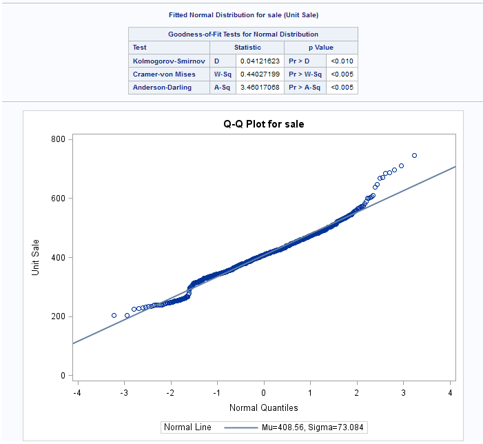
Checking for Normality Note: If you select any of these options, you can also specify whether to include these inset statistics: number of observations, goodness-of-fit test, mean, median, standard deviation, variance, skewness, and kurtosis.
Histogram and goodness-of-fit tests	requests tests for normality that include a series of goodness-of-fit tests based on the empirical distribution function. The table provides test statistics and p-values for the Shapiro-Wilk test (provided the sample size is less than or equal to 2,000), the Kolmogorov-Smirnov test, the Anderson-Darling test, and the Cramér-von Mises test.
Normal probability plot	creates a probability plot, which compares ordered variable values with the percentiles of the normal distribution. If the data distribution matches the normal distribution, the points on the plot form a linear pattern. Probability plots are preferable for graphical estimation of percentiles. The distribution reference line on the plot is created from the maximum likelihood estimate for the parameter. You can also specify whether to include an inset box of selected statistics in the graph.
Normal quantile-quantile plot	creates quantile-quantile plots (Q-Q plots) and compares ordered variable values with quantiles of the normal distribution. If the data distribution matches the normal distribution, the points on the plot form a linear pattern. Q-Q plots are preferable for graphical estimation of distribution parameters. The distribution reference line on the plot is created from the maximum likelihood estimate for the parameter. You can also specify whether to include an inset box of selected statistics in the graph.
Fitting Distributions Note: If you select a plot option for any of these distributions, you can also specify whether to include these inset statistics: number of observations, mean, median, standard deviation, and variance.
Beta
Histogram and goodness-of-fit tests	fits beta distribution with threshold parameter , scale parameter , and shape parameters and .
Probability plot	specifies a beta probability plot for shape parameters and .
Quantile-quantile plot	specifies a beta Q-Q plot for shape parameters and .
Exponential
Histogram and goodness-of-fit tests	fits exponential distribution with threshold parameter and scale parameter .
Probability plot	specifies an exponential probability plot.
Quantile-quantile plot	specifies an exponential Q-Q plot.
Gamma
Histogram and goodness-of-fit tests	fits gamma distribution with threshold parameter , scale parameter , and shape parameter .
Probability plot	specifies a gamma probability plot for shape parameter .
Quantile-quantile plot	specifies a gamma Q-Q plot for shape parameter .
Lognormal
Histogram and goodness-of-fit tests	fits lognormal distribution with threshold parameter , scale parameter , and shape parameter .
Probability plot	specifies a lognormal probability plot for shape parameter .
Quantile-quantile plot	specifies a lognormal Q-Q plot for shape parameter .
Weibull
Histogram and goodness-of-fit tests	fits Weibull distribution with threshold parameter , scale parameter , and shape parameter .
Probability plot	specifies a two-parameter Weibull probability plot.
Quantile-quantile plot	specifies a two-parameter Weibull Q-Q plot.