Binary Logistic Regression Task

Assigning Data to Roles
To run the Binary Logistic
Regression task, you must assign columns to the Response
variable and a column to either the Classification
variables role or the Continuous variables role.
|
Role
|
Description
|
|---|---|
|
Roles
|
|
|
Response
|
|
|
Response
data consists of numbers of events and trials
|
specifies whether the
response data consists of events and trials.
|
|
Number of
events
|
specifies the variable
that contains the number of events for each observation.
|
|
Number of
trials
|
specifies the variable
that contains the number of trials for each observation.
|
|
Response
|
specifies the variable
that contains the response data. To perform a binary logistic regression,
the response variable should have only two levels.
Use the Event
of interest drop-down list to select the event category
for the binary response model.
|
|
Link function
|
specifies the link function
that links the response probabilities to the linear predictors.
Here are the valid
values:
|
|
Explanatory Variables
|
|
|
Classification
variables
|
specifies the classification
variables to use in the analysis. A classification variable is a variable
that enters the statistical analysis or model not through its values,
but through its levels. The process of associating values of a variable
with levels is termed levelization.
|
|
Parameterization of
Effects
|
|
|
Coding
|
specifies the parameterization
method for the classification variable. Design matrix columns are
created from the classification variables according to the selected
coding scheme.
You can select from
these coding schemes:
|
|
Treatment of Missing
Values
|
|
|
An observation is excluded
from the analysis when either of these conditions is met:
|
|
|
Continuous
variables
|
specifies the continuous
variables to use as the explanatory variables in the analysis.
|
|
Additional Roles
|
|
|
Frequency
count
|
specifies the variables
that contain the frequency of occurrence for each observation. The
task treats each observation as if it appears n times,
where n is the value of the variable for that
observation.
|
|
Weight variable
|
specifies the how much
to weight each observation in the input data set.
|
|
Group analysis
by
|
creates separate analyses
based on the number of BY variables.
|
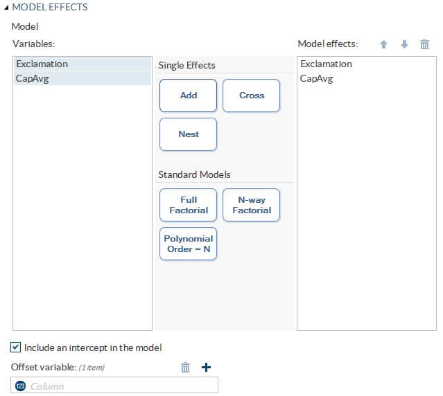
Building a Model
Create a Nested Effect
Nested effects are specified
by following a main effect or crossed effect with a classification
variable or list of classification variables enclosed in parentheses.
The main effect or crossed effect is nested within the effects listed
in parentheses. Here are examples of nested effects: B(A), C(B*A),
D*E(C*B*A). In this example, B(A) is read "A nested within B."
Create N-Way Factorial
For example, if you
select the Height, Weight, and Age variables and then specify the
value of N as 2, when you click N-way Factorial,
these model effects are created: Age, Height, Weight, Age*Height,
Age*Weight, and Height*Weight. If N is set to a value greater than
the number of variables in the model, N is effectively set to the
number of variables.
Create Polynomial Effects of the Nth Order
Setting the Model Options
|
Option
|
Description
|
|---|---|
|
Model
|
|
|
Include
an intercept in the model
|
specifies whether to
include the intercept in the model.
|
|
Offset variable
|
specifies a variable
to be used as an offset to the linear predictor. An offset plays the
role of an effect whose coefficient is known to be 1. Observations
that have missing values for the offset variable are excluded from
the analysis.
|
Specifying the Model Selection Options
|
Option
|
Description
|
|---|---|
|
Model Selection
|
|
|
Selection
method
|
specifies the model
selection method for the model. The task performs model selection
by examining whether effects should be added to or removed from the
model according to the rules that are defined by the selection method.
Here are the valid values
for the selection methods:
|
|
Selection
method (continued)
|
|
|
Details
|
|
|
Display
selection process details
|
specifies how much information
about the selection process to include in the results. You can choose
to display a summary, details for each step of the selection process,
or all of the information about the selection process.
|
|
Maintain
hierarchy of effects
|
specifies how the model
hierarchy requirement is applied and that only a single effect or
multiple effects can enter or leave the model at one time. For example,
suppose you specify the main effects A and B and the interaction A*B
in the model. In the first step of the selection process, either A
or B can enter the model. In the second step, the other main effect
can enter the model. The interaction effect can enter the model only
when both main effects have already been entered. Also, before A or
B can be removed from the model, the A*B interaction must first be
removed.
Model hierarchy refers
to the requirement that, for any term to be in the model, all effects
contained in the term must be present in the model. For example, in
order for the interaction A*B to enter the model, the main effects
A and B must be in the model. Likewise, neither effect A nor B can
leave the model while the interaction A*B is in the model.
|
Setting Options
|
Option Name
|
Description
|
|---|---|
|
Statistics
Note: In addition to the default
statistics that are included in the results, you can select the additional
statistics to include.
|
|
|
Classification
table
|
classifies the input
binary response observations according to whether the predicted event
probabilities are above or below the cut-point value z in
the range. An observation is predicted as an event if the predicted
event probability equals or exceeds z.
|
|
Partial
correlation
|
computes the partial
correlation statistic
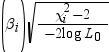 for each parameter i, where X2i is
the Wald chi-square statistic for the parameter and log
L0 is the log-likelihood of the
intercept-only model (Hilbe 2009). If X2i <
2, the partial correlation is set to 0. for each parameter i, where X2i is
the Wald chi-square statistic for the parameter and log
L0 is the log-likelihood of the
intercept-only model (Hilbe 2009). If X2i <
2, the partial correlation is set to 0.
|
|
Generalized
R square
|
requests a generalized
R square measure for the fitted model.
|
|
Goodness-of-fit and
Overdispersion
|
|
|
Deviance
and Pearson goodness-of-fit
|
specifies whether to
calculate the deviance and Pearson goodness-of-fit.
|
|
Aggregate
by
|
specifies the subpopulations
on which the Pearson chi-square test statistic and the likelihood
ratio chi-square test statistic (deviance) are calculated. Observations
with common values in the given list of variables are regarded as
coming from the same subpopulation. Variables in the list can be any
variables in the input data set.
|
|
Correct
for overdispersion
|
specifies whether to
correct for overdispersion by using the Deviance or Pearson estimate.
|
|
Hosmer &
Lemeshow goodness-of-fit
|
performs the Hosmer
and Lemeshow goodness-of-fit test (Hosmer and Lemeshow 2000) for the
case of a binary response model. The subjects are divided into approximately
10 groups of approximately the same size based on the percentiles
of the estimated probabilities. The discrepancies between the observed
and expected number of observations in these groups are summarized
by the Pearson chi-square statistic. This statistic is then compared
to a chi-square distribution with t degrees
of freedom, where t is the number of groups
minus n. By default, n =
2. A small p-value suggests that the fitted
model is not an adequate model.
|
|
Multiple Comparisons
|
|
|
Perform
multiple comparisons
|
specifies whether to
compute and compare the least squares means of fixed effects.
|
|
Select the
effects to test
|
specifies the effects
that you want to compare. You specified these effects on the Model tab.
|
|
Method
|
requests a multiple
comparison adjustment for the p-values and
confidence limits for the differences of the least squares means.
Here are the valid methods: Bonferroni, Nelson, Scheffé, Sidak,
and Tukey.
|
|
Significance
level
|
requests that a t type
confidence interval be constructed for each of the least squares means
with a confidence level of 1 – number.
The value of number must be
between 0 and 1. The default value is 0.05.
|
|
Exact Tests
|
|
|
Exact test
of intercept
|
calculates the exact
test for the intercept.
|
|
Select effects
to test
|
calculates exact tests
of the parameters for the selected effects.
|
|
Significance
level
|
specifies the level
of significance
 for for  confidence limits for the parameters or odds ratios. confidence limits for the parameters or odds ratios.
|
|
Parameter Estimates
|
|
|
You can calculate these
parameter estimates:
You can specify the
confidence intervals for parameters, confidence intervals for odds
ratios, and the confidence level for these estimates.
|
|
|
Diagnostics
|
|
|
Influence
diagnostics
|
displays the diagnostic
measures for identifying influential observations. For each observation,
the results include the sequence number of the observation, the values
of the explanatory variables included in the final model, and the
regression diagnostic measures developed by Pregibon (1981). You can
specify whether to include the standardized and likelihood residuals
in the results.
|
|
Plots
|
|
|
You can select whether
to include plots in the results.
Here are the additional
plots that you can include in the results:
You can specify whether
to display these plots in a panel or individually.
|
|
|
Label influence
and ROC plots
|
specifies the variable
from the input data that contains the labels for the influence and
ROC plots.
|
|
Maximum
number of plot points
|
specifies the maximum
number of points to include in the plots. By default, 5,000 points
are shown.
|
|
Methods
|
|
|
Optimization
|
|
|
Method
|
specifies the optimization
technique for estimating the regression parameters. The Fisher scoring
and Newton-Raphson algorithms yield the same estimates, but the estimated
covariance matrices are slightly different except when the Logit link
function is specified for binary response data.
|
|
Maximum
number of iterations
|
specifies the maximum
number of iterations to perform. If convergence is not attained in
a specified number of iterations, the displayed output and all output
data sets created by the task contain results that are based on the
last maximum likelihood iteration.
|
Creating Output Data Sets
|
Option Name
|
Description
|
|---|---|
|
Output Data Sets
|
|
|
You can create two types
of output data sets. Select the check box for each data set that you
want to create.
Create output data set
outputs a data set
that contains the specified statistics.
Here are the statistics
that you can include in the output data set:
Create scored data set
outputs a data set
that contains all the statistics in the output data set plus posterior
probabilities.
|
|
|
Add SAS
scoring code to the log
|
writes SAS DATA step
code for computing predicted values of the fitted model either to
a file or to a catalog entry. This code can then be included in a
DATA step to score new data.
|
Copyright © SAS Institute Inc. All rights reserved.