Linear Regression Task
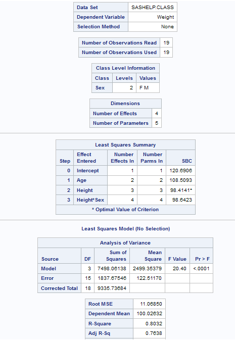
Example: Predicting Weight Based on a Student’s Height

Assigning Data to Roles
To run the Linear Regression
task, you must assign a column to the Dependent variable role
and a column to the Classification variables role
or the Continuous variables role.
|
Role
|
Description
|
|---|---|
|
Roles
|
|
|
Dependent
variable
|
specifies the numeric
variable to use as the dependent variable for the regression analysis.
You must assign a numeric variable to this role.
|
|
Classification
variables
|
specifies categorical
variables that enter the regression model through the design matrix
coding.
|
|
Parameterization of
Effects
|
|
|
Coding
|
specifies the parameterization
method for the classification variable. Design matrix columns are
created from the classification variables according to the selected
coding scheme.
You can select from
these coding schemes:
|
|
Treatment of Missing
Values
|
|
|
An observation is excluded
from the analysis when either of these conditions is met:
|
|
|
Continuous
variables
|
specifies the numeric
covariates (regressors) for the regression model.
|
|
Additional Roles
|
|
|
Frequency
count
|
lists a numeric variable
whose value represents the frequency of the observation. If you assign
a variable to this role, the task assumes that each observation represents n observations,
where n is the value of the frequency variable.
If n is not an integer, SAS truncates it. If n is
less than 1 or is missing, the observation is excluded from the analysis.
The sum of the frequency variable represents the total number of observations.
|
|
Weight
|
specifies the variable
to use as a weight to perform a weighted analysis of the data.
|
|
Group analysis
by
|
specifies to create
a separate analysis for each group of observations.
|
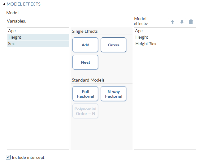
Building a Model
Requirements for Building a Model
To specify an effect,
you must assign at least one column to the Classification
variables role or the Continuous variables role.
You can select combinations of variables to create crossed, nested,
factorial, or polynomial effects. You can also specify whether to
include the intercept in the model.
To create the model,
use the model builder on the Model tab.
Create a Nested Effect
Nested effects are specified
by following a main effect or crossed effect with a classification
variable or list of classification variables enclosed in parentheses.
The main effect or crossed effect is nested within the effects listed
in parentheses. Here are examples of nested effects: B(A), C(B*A),
D*E(C*B*A). In this example, B(A) is read "A nested within B."
Create N-Way Factorial
For example, if you
select the Height, Weight, and Age variables and then specify the
value of N as 2, when you click N-way Factorial,
these model effects are created: Age, Height, Weight, Age*Height,
Age*Weight, and Height*Weight. If N is set to a value greater than
the number of variables in the model, N is effectively set to the
number of variables.
Setting the Model Options
|
Option Name
|
Description
|
|---|---|
|
Methods
|
|
|
Confidence
level
|
specifies the significance
level to use for the construction of confidence intervals.
|
|
Statistics
|
|
|
You can choose to include
the default statistics in the results or choose to include additional
statistics.
|
|
|
Additional available
statistics
|
|
|
Parameter Estimates
|
|
|
Standardized
regression coefficients
|
displays the standardized
regression coefficients. A standardized regression coefficient is
computed by dividing a parameter estimate by the ratio of the sample
standard deviation of the dependent variable to the sample standard
deviation of the regressor.
|
|
Confidence
limits for estimates
|
displays the
 upper and lower confidence limits for the parameter
estimates. upper and lower confidence limits for the parameter
estimates.
|
|
Sums of Squares
|
|
|
Sequential
sum of squares (Type I)
|
displays the sequential
sums of squares (Type I SS) along with the parameter estimates for
each term in the model.
|
|
Partial
sum of squares (Type II)
|
displays the partial
sums of squares (Type II SS) along with the parameter estimates for
each term in the model.
|
|
Partial and Semipartial
Correlations
|
|
|
Squared
partial correlations
|
displays the squared
partial correlation coefficients computed by using Type I and Type
II sums of squares.
|
|
Squared
semipartial correlations
|
displays the squared
semipartial correlation coefficients computed by using Type I and
Type II sums of squares. This value is calculated as sum of squares
divided by the corrected total sum of squares.
|
|
Diagnostics
|
|
|
Analysis
of influence
|
requests a detailed
analysis of the influence of each observation on the estimates and
the predicted values.
|
|
Analysis
of residuals
|
requests an analysis
of the residuals. The results include the predicted values from the
input data and the estimated model, the standard errors of the mean
predicted and residual values, the studentized residual, and Cook’s D statistic
to measure the influence of each observation on the parameter estimates.
|
|
Predicted
values
|
calculates predicted
values from the input data and the estimated model.
|
|
Multiple Comparisons
|
|
|
Perform
multiple comparisons
|
specifies whether to
compute and compare the least squares means of fixed effects.
|
|
Select the
effects to test
|
specifies the effects
that you want to compare. You specified these effects on the Model tab.
|
|
Method
|
requests a multiple
comparison adjustment for the p-values and
confidence limits for the differences of the least squares means.
Here are the valid methods: Bonferroni, Nelson, Scheffé, Sidak,
and Tukey.
|
|
Significance
level
|
requests that a t type
confidence interval be constructed for each of the least squares means
with a confidence level of 1 – number. The value of number
must be between 0 and 1. The default value is 0.05.
|
|
Collinearity
|
|
|
Collinearity
analysis
|
requests a detailed
analysis of collinearity among the regressors. This includes eigenvalues,
condition indices, and decomposition of the variances of the estimates
with respect to each eigenvalue.
|
|
Tolerance
values for estimates
|
produces tolerance values
for the estimates. Tolerance for a variable is defined as
 , where R square is obtained from the regression
of the variable on all other regressors in the model. , where R square is obtained from the regression
of the variable on all other regressors in the model.
|
|
Variance
inflation factors
|
produces variance inflation
factors with the parameter estimates. Variance inflation is the reciprocal
of tolerance.
|
|
Heteroscedasticity
|
|
|
Heteroscedasticity
analysis
|
performs a test to confirm
that the first and second moments of the model are correctly specified.
|
|
Asymptotic
covariance matrix
|
displays the estimated
asymptotic covariance matrix of the estimates under the hypothesis
of heteroscedasticity and heteroscedasticity-consistent standard errors
of parameter estimates.
|
|
Plots
|
|
|
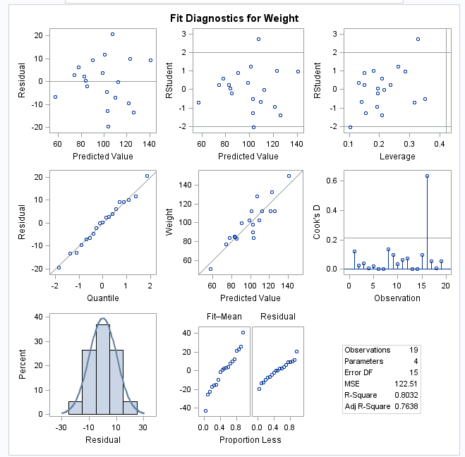
Diagnostic and Residual
Plots
|
|
|
By default, several
diagnostic plots are included in the results. You can also specify
whether to include plots of the residuals for each explanatory variable.
|
|
|
More Diagnostic Plots
|
|
|
Rstudent
statistic by predicted values
|
plots studentized residuals
by predicted values. If you select the Label extreme points option,
observations with studentized residuals that lie outside the band
between the reference lines
 are deemed outliers. are deemed outliers.
|
|
DFFITS statistic
by observations
|
plots the DFFITS statistic
by observation number. If you select the Label extreme
points option, observations with a DFFITS statistic greater
in magnitude than
 are deemed influential. The number of observations
used is n, and the number of regressors is p. are deemed influential. The number of observations
used is n, and the number of regressors is p.
|
|
DFBETAS
statistic by observation number for each explanatory variable
|
produces panels of DFBETAS
by observation number for the regressors in the model. You can view
these plots as a panel or as individual plots. If you select the Label
extreme points option, observations with a DFBETAS statistic
greater in magnitude than
 are deemed influential for that regressor. The number
of observations used is n. are deemed influential for that regressor. The number
of observations used is n.
|
|
Label extreme
points
|
identifies the extreme
values on each different type of plot.
|
|
Scatter Plots
|
|
|
Fit plot
for a single continuous variable
|
produces a scatter plot
of the data overlaid with the regression line, confidence band, and
prediction band for models with a single continuous variable. The
intercept is excluded. When the number of points exceeds the value
for the Maximum number of plot points option,
a heat map is displayed instead of a scatter plot.
|
|
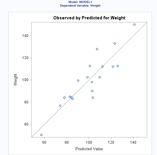
Observed
values by predicted values
|
produces a scatter plot
of the observed values versus the predicted values.
|
|
Partial
regression plots for each explanatory variable
|
produces partial regression
plots for each regressor. If you display these plots in a panel, there
is a maximum of six regressors per panel.
|
|
Maximum
number of plot points
|
specifies the maximum
number of points to include in each plot.
|
Setting the Model Selection Options
|
Option
|
Description
|
|---|---|
|
Model Selection
|
|
|
Selection
method
|
specifies the model
selection method for the model. The task performs model selection
by examining whether effects should be added to or removed from the
model according to the rules that are defined by the selection method.
Here are the valid values
for the selection methods:
|
|
Criterion
to add or remove effects
|
specifies the criterion
to use to add or remove effects from the model.
|
|
Criterion
to stop adding or removing effects
|
specifies the criterion
to use to stop adding or removing effects from the model.
|
|
Select best
model by
|
specifies the criterion
to use to identify the best fitting model.
|
|
Selection Statistics
|
|
|
Model fit
statistics
|
specifies which model
fit statistics are displayed in the fit summary table and the fit
statistics tables. If you select Default fit statistics,
the default set of statistics that are displayed in these tables includes
all the criteria used in model selection.
Here are the additional
fit statistics that you can include in the results:
|
|
Selection Plots
|
|
|
Criterion
plots
|
displays plots for these
criteria: adjusted R-square, Akaike’s information criterion,
Akaike’s information criterion corrected for small-sample bias,
and the criterion used to select the best fitting model.
|
|
Coefficient
plots
|
displays these plots:
|
|
Details
|
|
|
Selection
process details
|
specifies how much information
about the selection process to include in the results. You can display
a summary, details for each step of the selection process, or all
of the information about the selection process.
|
Creating Output Data Sets
You can specify whether
to create an observationwise statistics data set. This data set contains
the sum of squares and cross-products.
You can also choose
to include these statistics in the output data set:
-
Cook’s D influence
-
the standard influence of observation on covariance of betas
-
the standard influence of an observation on predicted value (called DFFITS)
-
leverage
-
predicted values
-
press statistic, which is the ith residual divided by
 , where h is the leverage,
and where the model has been refit without the ith
observation
, where h is the leverage,
and where the model has been refit without the ith
observation
-
residual
-
studentized residuals, which are the residuals divided by their standard errors
-
studentized residual with current observation removed
Copyright © SAS Institute Inc. All rights reserved.