Predictive Regression Model :: SAS(R) Studio 3.3: User's Guide

About the Predictive Regression Model

The task is predictive in that it selects the most influential effects based on observed data. This task enables you to logically partition your data into disjoint subsets for model training, validation, and testing. The Predictive Regression Model task focuses on the standard independently and identically distributed general linear model for univariate responses and offers great flexibility and insight into the model selection algorithm. This task can also create a scored data set. The results for this task make it easy to explore the selected model in more detail with other tasks, such as the Linear Regression task.

Example: Predicting a Baseball Player’s Salary

To create this example:

In the Tasks section, expand the Statistics folder and double-click Predictive Regression Model. The user interface for the Predictive Regression Model task opens.
On the Data tab, select the SASHELP.BASEBALL data set.

Assign columns to these roles and specify these options:

Role	Column Name
Dependent variable	logSalary
Classification variables	League Division
Continuous variables	nAtBat nHits nHome nRuns nRBI nBB

Click the Model tab. Select the nAtBat, nHits, nHome, nRuns, nRBI, nBB. League, and Division variables, and then click Add.
To run the task, click .

Subset of Results from Predictive Regression Model Task

Partitioning Your Data

When you have sufficient data, you can partition your data into three parts: training data, validation data, and test data. During the selection process, models are fit on the training data, and the prediction error for the model is determined using the validation data. This prediction error can be used to decide when to terminate the selection process or which effects to include as the selection process proceeds. Finally, after a model is selected, the test data can be used to assess how the selected model generalizes on data that played no role in selecting the model.

You can partition your data in either of these ways:

You can specify a proportion of the validation or test data. The proportions are used to divide the input data by sampling.
If the input data set contains a variable whose values indicate whether an observation is a validation or test case, you can specify the variable to use when partitioning the data. When you specify the variable, you also select the appropriate values for validation or test cases. The input data set is divided into partitions by using these values.

Assigning Data to Roles

To run the Predictive Regression Model task, you must assign a column to the Dependent variable role and a column to the Classification variables role or the Continuous variables role.

Role	Description
Roles
Dependent variable	specifies the numeric variable to use as the dependent variable for the regression analysis.
Classification variables	specifies the variables to use to group (classify) data in the analysis. A classification variable is a variable that enters the statistical analysis or model through its levels, not through its values. The process of associating values of a variable with levels is termed levelization.
Parameterization of Effects
Coding	specifies the parameterization method for the classification variable. Design matrix columns are created from the classification variables according to the selected coding scheme. You can select from these coding schemes: Effects coding specifies effect coding. GLM coding specifies less-than-full-rank, reference-cell coding. This coding scheme is the default. Reference coding specifies reference-cell coding.
Treatment of Missing Values
An observation is excluded from the analysis if any variable in the model contains a missing value. In addition, an observation is excluded if any classification variable specified earlier in this table contains a missing value, regardless if it is used in the model.
Continuous variables	specifies the independent covariates (regressors) for the regression model. If you do not specify a continuous variable, the task fits a model that contains only an intercept.
Additional Roles
Frequency count	lists a numeric variable whose value represents the frequency of the observation. If you assign a variable to this role, the task assumes that each observation represents n observations, where n is the value of the frequency variable. If n is not an integer, SAS truncates it. If n is less than 1 or is missing, the observation is excluded from the analysis. The sum of the frequency variable represents the total number of observations.
Weight	specifies the numeric column to use as a weight to perform a weighted analysis of the data.
Group analysis by	specifies to create a separate analysis for each group of observations.

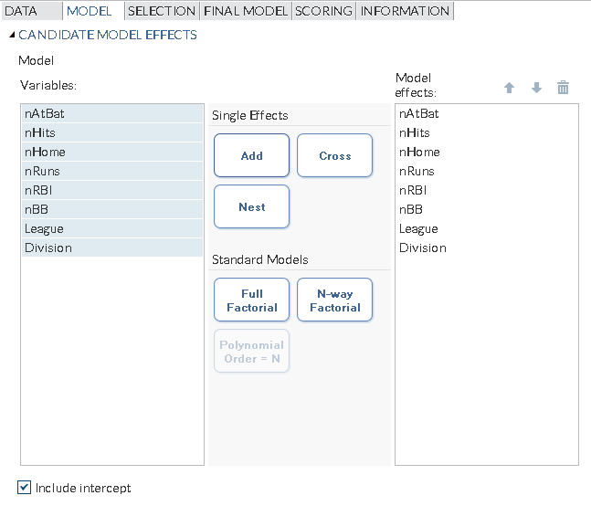
Building a Model

Requirements for Building a Model

To specify an effect, you must assign at least one column to the Classification variables role or the Continuous variables role. You can select combinations of variables to create crossed, factorial, or polynomial effects.

To create a model, use the model builder on the Model tab. After you create a model, you can specify whether to include the intercept in the model.

Create a Main Effect

Select the variable name in the Variables box.
Click Add to add the variable to the Model effects box.

Create Crossed Effects (Interactions)

Select two or more variables in the Variables box. To select more than one variable, press Ctrl.
Click Cross.

Create a Nested Effect

Nested effects are specified by following a main effect or crossed effect with a classification variable or list of classification variables enclosed in parentheses. The main effect or crossed effect is nested within the effects listed in parentheses. Here are examples of nested effects: B(A), C(B*A), D*E(C*B*A). In this example, B(A) is read "A nested within B."

Select the effect name in the Model effects box.
Click Nest. The Nested window opens.
Select the variable to use in the nested effect. Click Outer or Nested within Outer to specify how to create the nested effect.

Note: The Nested within Outer button is available only when a classification variable is selected.
Click Add.

Create a Full Factorial Model

Select two or more variables in the Variables box.
Click Full Factorial.

For example, if you select the Height, Weight, and Age variables and then click Full Factorial, these model effects are created: Age, Height, Weight, Age*Height, Age*Weight, Height*Weight, and Age*Height*Weight.

Create N-Way Factorial

Select two or more variables in the Variables box.
Click N-way Factorial to add these effects to the Model effects box.

For example, if you select the Height, Weight, and Age variables and then specify the value of N as 2, when you click N-way Factorial, these model effects are created: Age, Height, Weight, Age*Height, Age*Weight, and Height*Weight. If N is set to a value greater than the number of variables in the model, N is effectively set to the number of variables.

Create Polynomial Effects of the Nth Order

Select one variable in the Variables box.
Specify higher-degree crossings by adjusting the number in the N field.
Click Polynomial Order=N to add the polynomial effects to the Model effects box.

For example, if you select the Age and Height variables and then you specify 3 in the N field, when you click Polynomial Order=N, these model effects are created: Age, Age*Age, Age*Age*Age, Height, Height*Height, and Height*Height*Height.

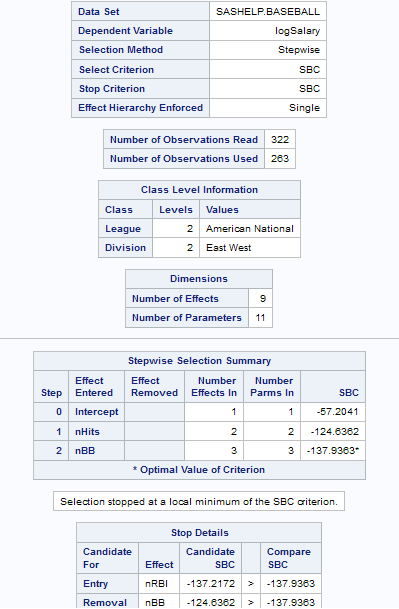
Selecting a Model

Option Name	Description
Model Selection
Selection method	By default, the complete model that you specified is used to fit the model. However, you can also use one of these selection methods:
Selection method (continued)	Forward selection specifies forward selection. This method starts with no effects in the model and adds effects. Backward elimination specifies backward elimination. This method starts with all effects in the model and deletes effects. Stepwise regression specifies stepwise regression, which is similar to the forward selection method except that effects already in the model do not necessarily stay there. LASSO specifies the LASSO method, which adds and deletes parameters based on a version of ordinary least squares where the sum of the absolute regression coefficients is constrained. If the model contains classification variables, these classification variables are split. Adaptive LASSO requests that adaptive weights be applied to each of the coefficients in the LASSO method. The ordinary least squares estimates of the parameters in the model are used in forming the adaptive weights.
Selection method (continued)	Elastic net specifies the elastic net method, which is an extension of LASSO. The elastic net method estimates parameters based on a version of ordinary least squares in which both the sum of the absolute regression coefficients and the sum of the squared regression coefficients are constrained. If the model contains classification variables, these classification variables are split. Least angle regression specifies least angle regression. This method starts with no effects in the model and adds effects. The parameter estimates at any step are “shrunk” when compared to the corresponding least squares estimates. If the model contains classification variables, these classification variables are split.
Criterion to add or remove effects	specifies the criterion to use to determine whether an effect should be added or removed from the model.
Criterion to stop adding or removing effects	specifies the criterion to use to determine whether effects should stop being added or removed from the model.
Select best model by	specifies the criterion to use to determine the best fitting model.
Selection Statistics
Model fit statistics	specifies which model fit statistics are displayed in the fit summary table and the fit statistics tables. If you select Default fit statistics, the default set of statistics that are displayed in these tables includes all the criteria used in model selection. Here are the additional fit statistics that you can include in the results: Adjusted R-square Akaike’s information criterion Akaike’s information criterion corrected for small-sample bias Average square error Bayesian information criterion Mallows’ Cp Press statistic, which specifies the predicted residual sum of squares statistic R-square Schwarz’s Bayesian information criterion
Selection Plots
Criterion plots	displays plots for these criteria: adjusted R-square, Akaike’s information criterion, Akaike’s information criterion corrected for small-sample bias, and the criterion used to select the best fitting model. You can choose to display these plots in a panel or individually.
Coefficient plots	displays these plots: a plot that shows the progression of the parameter values as the selection process proceeds a plot that shows the progression of the criterion used to select the best fitting model
Details
Selection process details	specifies how much information about the selection process to include in the results. You can display a summary, details for each step of the selection process, or all of the information about the selection process.
Model Effects Hierarchy
Model effects hierarchy	specifies how the model hierarchy requirement is applied and that only a single effect or multiple effects can enter or leave the model at one time. For example, suppose you specify the main effects A and B and the interaction AB in the model. In the first step of the selection process, either A or B can enter the model. In the second step, the other main effect can enter the model. The interaction effect can enter the model only when both main effects have already been entered. Also, before A or B can be removed from the model, the AB interaction must first be removed. Model hierarchy refers to the requirement that, for any term to be in the model, all effects contained in the term must be present in the model. For example, in order for the interaction AB to enter the model, the main effects A and B must be in the model. Likewise, neither effect A nor B can leave the model while the interaction AB is in the model.
Model effects subject to the hierarchy requirement	specifies whether to apply the model hierarchy requirement to the classification and continuous effects in the model or to only the classification effects.

Setting the Options for the Final Model

Option Name	Description
Statistics for the Selected Model
You can choose to include the default statistics in the results or choose to include additional statistics, such as the standardized regression coefficients. A standardized regression coefficient is computed by dividing a parameter estimate by the ratio of the sample standard deviation of the dependent variable to the sample standard deviation of the regressor.
Collinearity
Collinearity analysis	requests a detailed analysis of collinearity among the regressors. This includes eigenvalues, condition indices, and decomposition of the variances of the estimates with respect to each eigenvalue.
Tolerance values for estimates	produces tolerance values for the estimates. Tolerance for a variable is defined as , where R square is obtained from the regression of the variable on all other regressors in the model.
Variance inflation factors	produces variance inflation factors with the parameter estimates. Variance inflation is the reciprocal of tolerance.
Plots for the Selected Model
Diagnostic and Residual Plots
You must specify whether to include the default diagnostic plots in the results. You can also specify whether to include plots of the residuals for each explanatory variable.
More Diagnostic Plots
Rstudent statistic by predicted values	plots studentized residuals by predicted values. If you select the Label extreme points option, observations with studentized residuals that lie outside the band between the reference lines are deemed outliers.
DFFITS statistic by observation number	plots the DFFITS statistic by observation number. If you select the Label extreme points option, observations with a DFFITS statistic greater in magnitude than are deemed influential. The number of observations used is n, and the number of regressors is p.
DFBETAS statistic by observation number for each explanatory variable	produces panels of DFBETAS by observation number for the regressors in the model. You can view these plots as a panel or as individual plots. If you select the Label extreme points option, observations with a DFBETAS statistic greater in magnitude than $fraction 2 , over square root of n end fraction$ are deemed influential for that regressor. The number of observations used is n.
Label extreme points	identifies the extreme values on each different type of plot.
Scatter Plots
Observed values by predicted values	produces a scatter plot of the observed values versus the predicted values.
Partial regression plots for each explanatory variable	produces partial regression plots for each regressor. If you display these plots in a panel, there is a maximum of six regressors per panel.
Maximum number of plot points	specifies the maximum number of points to include in each plot.

Setting the Scoring Options

Option Name	Description
Scoring
You can create a scored data set, which contains the predicted values and the residuals.
Add SAS scoring code to the log	writes SAS DATA step code for computing predicted values of the fitted model either to a file or to a catalog entry. This code can then be included in a DATA step to score new data.