Model Fitting: Robust Regression

Example

The example in Chapter 21, "Model Fitting: Linear Regression," models 1987 salaries of Major League Baseball players as a function of several explanatory variables in the Baseball data set by using ordinary least squares regression. In that example, two conclusions are reached:

• no_home, the number of home runs is not a significant variable in the model.
• Several players are high leverage points. Pete Rose has the highest leverage because of his 25 years in the major leagues. Graig Nettles and Steve Sax are leverage points and also outliers.

However, the model fitted by using ordinary least squares is influenced by high leverage points and outliers. Robust regression is a preferable method of detecting influential observations. This example uses the Robust Regression analysis to identify leverage points and outliers in the Baseball data. This example models the logarithm of salary by using no_hits and yr_major as explanatory variables.

Open the Baseball data set.

The following two steps are the same as for the example in the section "Example" in Chapter 21, "Model Fitting: Linear Regression":

Use the Variable Transformation Wizard to create a new variable, Log10_salary, containing the logarithmic transformation of the salary variable.

Choose name to be the label variable for these data.

The following steps model Log10_salary as a function of two explanatory variables.

Select Analysis Model Fitting Robust Regression from the main menu, as shown in Figure 22.1.

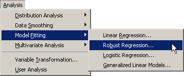
Figure 22.1: Selecting a Robust Regression

A dialog box appears as in Figure 22.2.

Scroll to the end of the variable list. Select the Log10_salary, and click Set Y.

Select no_hits. While holding down the CTRL key, select yr_major. Click Add X.

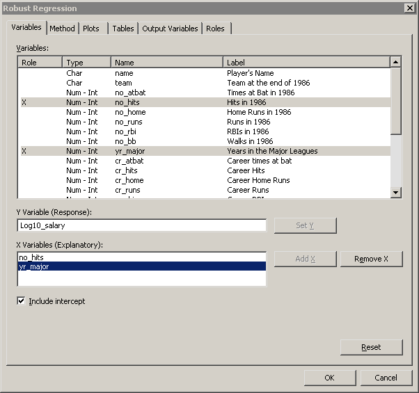
Figure 22.2: The Variables Tab

Click the Method tab.

The Method tab becomes active, as shown in Figure 22.3. There are four robust estimation methods. The default method, known as M estimation, is not robust in the presence of high leverage points. The LTS and MM methods are better suited for handling high leverage points.

Select MM for the method.

Note: If you use M estimation on data that contain leverage points, the ROBUSTREG procedure prints the following message to the error log:

WARNING: The data set contains one or more high leverage points, for which M estimation is not robust. It is recommended that you use METHOD=LTS or METHOD=MM for this data set.

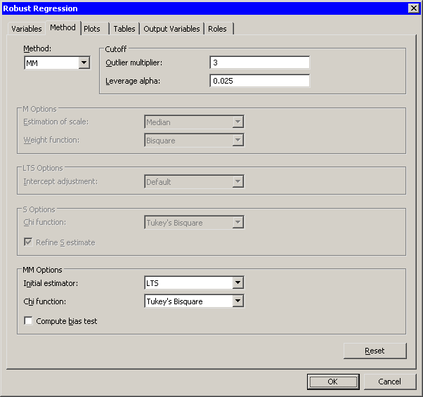
Figure 22.3: The Method Tab

Click the Plots tab.

The Plots tab becomes active, as shown in Figure 22.4. This tab controls which graphs are produced by the analysis. One plot is selected by default. For this example, select the following additional plots:

Select Observed vs. Predicted.

Select Robust residuals vs. Predicted.

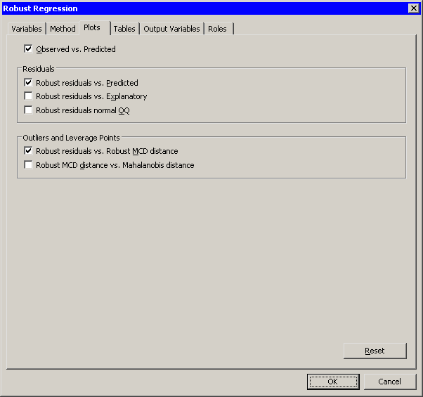
Figure 22.4: The Plots Tab

Click the Output Variables tab.

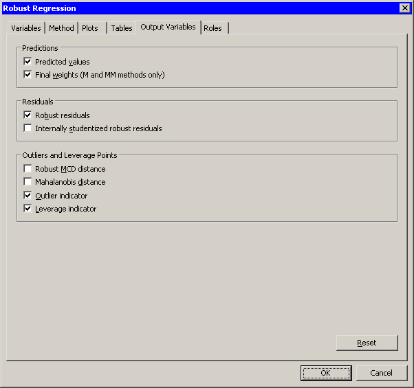
The Output Variables tab becomes active, as shown in Figure 22.5. This tab controls which analysis variables are added to the data table.

Select Final Weights (M and MM methods only).

Note that the Outlier indicator and Leverage indicator options are selected by default. These options create indicator variables in the data table that you can use to identify outliers and leverage points.

Figure 22.5: The Output Variables Tab

Click OK to run the analysis.

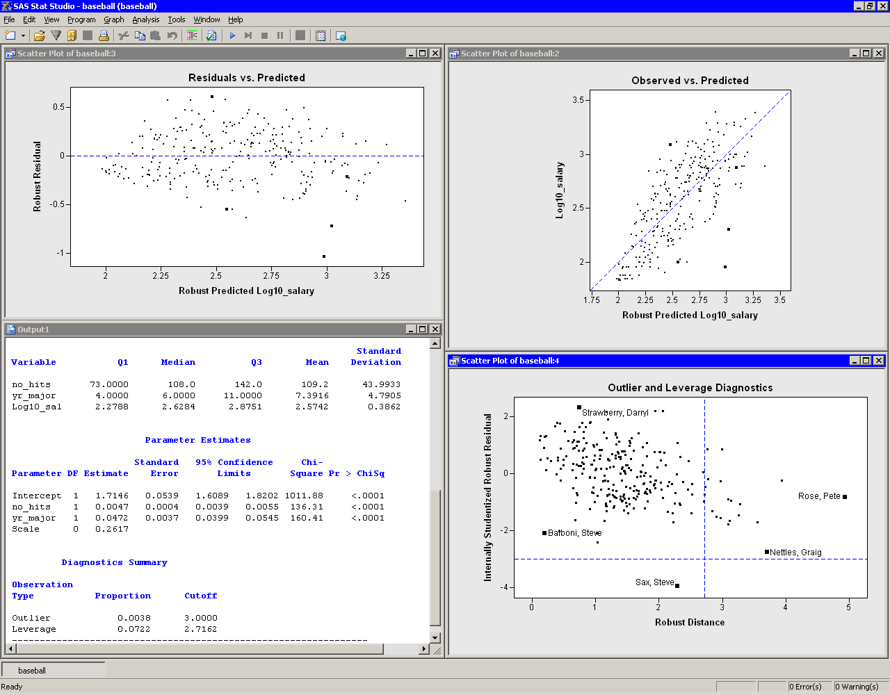
Several plots appear, along with output from the ROBUSTREG procedure. Some plots might be hidden beneath others. Move the windows so that they are arranged as in Figure 22.6. In the figure, five players are selected to facilitate comparison with Figure 21.9 and Figure 21.12.

The plots involving predicted values are similar to those in Figure 21.9. The plot of residuals versus predicted values does not show any obvious trends. The plot of observed versus predicted values shows a reasonable fit, with a few exceptions.

The plot of (internally) studentized robust residuals versus robust distance (known as an RD plot) identifies which observations are outliers and which are high leverage points. Observations outside the horizontal lines at are outliers; observations to the right of the vertical line at 2.7162 are leverage points. The values of the outlier and leverage cutoffs are displayed in the "Diagnostics Summary" table in the output window. You can control these values from the Method tab.

The robust regression model identifies Steve Sax as an outlier and identifies 19 other players (including Pete Rose and Graig Nettles) as leverage points. As displayed in the "Diagnostics Summary" table, these 19 players represent 7.2% of the 263 observations used in the analysis. (For comparison, the analysis in Chapter 21, "Model Fitting: Linear Regression," suggests 11 outliers and 16 leverage points.)

Figure 22.6: Results from the Robust Regression Analysis

---

Using the Results of Robust Regression