The VARIOGRAM Procedure

Semivariance Computation

With the classification of a point pair $P_ iP_ j$ into an angle/distance class, as shown earlier in this section, the semivariance computation proceeds as follows.

Denote all pairs that $P_ iP_ j$ belong to angle class $[\theta _ k-\delta \theta _ k,\theta _ k+\delta \theta _ k)$ and distance class $L=L(P_ iP_ j)$ as $N(\theta _ k,L)$ . For example, based on Figure 122.20 and Figure 122.21, $P_1P_2$ belongs to $N(60^{\circ },1)$ .

Let $\mid N(\theta _ k,L) \mid$ denote the number of such pairs. The component of the standard (or method of moments) semivariance that correspond to angle/distance class $N(\theta _ k,L)$ is given by

$\hat{\gamma }(h_ k) = \frac{1}{2 \mid N(\theta _ k,L) \mid } \sum _{P_ iP_ j \in N(\theta _ k,L)}[V(\bm {s}_ i)-V(\bm {s}_ j)]^2$

where $h_ k$ is the average distance in class $N(\theta _ k,L)$ ; that is,

$h_ k = \frac{1}{\mid N(\theta _ k,L) \mid }\sum _{P_ iP_ j \in N(\theta _ k,L)}\mid P_ iP_ j \mid$

The robust version of the semivariance is given by

$\bar{\gamma }(h_ k) = \frac{\Psi ^4(h_ k)}{2 [0.457 + 0.494/N(\theta _ k,L)]}$

where

$\Psi (h_ k) = \frac{1}{N(\theta _ k,L)} \sum _{P_ iP_ j \in N(\theta _ k,L)}[V(\bm {s}_ i)-V(\bm {s}_ j)]^{\frac{1}{2}}$

This robust version of the semivariance is computed when you specify the ROBUST option in the COMPUTE statement in PROC VARIOGRAM.

PROC VARIOGRAM computes and writes to the OUTVAR= data set the quantities 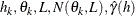$h_ k, \theta _ k, L, N(\theta _ k,L), \hat{\gamma }(h)$ , and $\bar{\gamma }(h)$ .