The PRINCOMP Procedure

Getting Started: PRINCOMP Procedure

The following data provide crime rates per 100,000 people in seven categories for each of the 50 US states in 1977. Because there are seven numeric variables, it is impossible to plot all the variables simultaneously. You can use principal components to summarize the data in two or three dimensions, and they help you visualize the data. The following statements produce Figure 91.1 through Figure 91.5:

title 'Crime Rates per 100,000 Population by State';

data Crime;
   input State $1-15 Murder Rape Robbery Assault
         Burglary Larceny Auto_Theft;
   datalines;
Alabama        14.2 25.2  96.8 278.3 1135.5 1881.9 280.7
Alaska         10.8 51.6  96.8 284.0 1331.7 3369.8 753.3
Arizona         9.5 34.2 138.2 312.3 2346.1 4467.4 439.5
Arkansas        8.8 27.6  83.2 203.4  972.6 1862.1 183.4
California     11.5 49.4 287.0 358.0 2139.4 3499.8 663.5
Colorado        6.3 42.0 170.7 292.9 1935.2 3903.2 477.1
Connecticut     4.2 16.8 129.5 131.8 1346.0 2620.7 593.2
Delaware        6.0 24.9 157.0 194.2 1682.6 3678.4 467.0
Florida        10.2 39.6 187.9 449.1 1859.9 3840.5 351.4
Georgia        11.7 31.1 140.5 256.5 1351.1 2170.2 297.9
Hawaii          7.2 25.5 128.0  64.1 1911.5 3920.4 489.4
Idaho           5.5 19.4  39.6 172.5 1050.8 2599.6 237.6
Illinois        9.9 21.8 211.3 209.0 1085.0 2828.5 528.6
Indiana         7.4 26.5 123.2 153.5 1086.2 2498.7 377.4
Iowa            2.3 10.6  41.2  89.8  812.5 2685.1 219.9
Kansas          6.6 22.0 100.7 180.5 1270.4 2739.3 244.3
Kentucky       10.1 19.1  81.1 123.3  872.2 1662.1 245.4
Louisiana      15.5 30.9 142.9 335.5 1165.5 2469.9 337.7
Maine           2.4 13.5  38.7 170.0 1253.1 2350.7 246.9
Maryland        8.0 34.8 292.1 358.9 1400.0 3177.7 428.5
Massachusetts   3.1 20.8 169.1 231.6 1532.2 2311.3 1140.1
Michigan        9.3 38.9 261.9 274.6 1522.7 3159.0 545.5
Minnesota       2.7 19.5  85.9  85.8 1134.7 2559.3 343.1
Mississippi    14.3 19.6  65.7 189.1  915.6 1239.9 144.4
Missouri        9.6 28.3 189.0 233.5 1318.3 2424.2 378.4
Montana         5.4 16.7  39.2 156.8  804.9 2773.2 309.2
Nebraska        3.9 18.1  64.7 112.7  760.0 2316.1 249.1
Nevada         15.8 49.1 323.1 355.0 2453.1 4212.6 559.2
New Hampshire   3.2 10.7  23.2  76.0 1041.7 2343.9 293.4
New Jersey      5.6 21.0 180.4 185.1 1435.8 2774.5 511.5
New Mexico      8.8 39.1 109.6 343.4 1418.7 3008.6 259.5
New York       10.7 29.4 472.6 319.1 1728.0 2782.0 745.8
North Carolina 10.6 17.0  61.3 318.3 1154.1 2037.8 192.1
North Dakota    0.9  9.0  13.3  43.8  446.1 1843.0 144.7
Ohio            7.8 27.3 190.5 181.1 1216.0 2696.8 400.4
Oklahoma        8.6 29.2  73.8 205.0 1288.2 2228.1 326.8
Oregon          4.9 39.9 124.1 286.9 1636.4 3506.1 388.9
Pennsylvania    5.6 19.0 130.3 128.0  877.5 1624.1 333.2
Rhode Island    3.6 10.5  86.5 201.0 1489.5 2844.1 791.4
South Carolina 11.9 33.0 105.9 485.3 1613.6 2342.4 245.1
South Dakota    2.0 13.5  17.9 155.7  570.5 1704.4 147.5
Tennessee      10.1 29.7 145.8 203.9 1259.7 1776.5 314.0
Texas          13.3 33.8 152.4 208.2 1603.1 2988.7 397.6
Utah            3.5 20.3  68.8 147.3 1171.6 3004.6 334.5
Vermont         1.4 15.9  30.8 101.2 1348.2 2201.0 265.2
Virginia        9.0 23.3  92.1 165.7  986.2 2521.2 226.7
Washington      4.3 39.6 106.2 224.8 1605.6 3386.9 360.3
West Virginia   6.0 13.2  42.2  90.9  597.4 1341.7 163.3
Wisconsin       2.8 12.9  52.2  63.7  846.9 2614.2 220.7
Wyoming         5.4 21.9  39.7 173.9  811.6 2772.2 282.0
;

ods graphics on;

proc princomp out=Crime_Components plots= score(ellipse ncomp=3);
   id State;
run;

Figure 91.1 displays the PROC PRINCOMP output, beginning with simple statistics and followed by the correlation matrix. By default, the PROC PRINCOMP statement requests principal components that are computed from the correlation matrix, so the total variance is equal to the number of variables, 7.

Figure 91.1: Number of Observations and Simple Statistics from the PRINCOMP Procedure

Crime Rates per 100,000 Population by State

The PRINCOMP Procedure

Observations	50
Variables	7

Simple Statistics
	Murder	Rape	Robbery	Assault	Burglary	Larceny	Auto_Theft
Mean	7.444000000	25.73400000	124.0920000	211.3000000	1291.904000	2671.288000	377.5260000
StD	3.866768941	10.75962995	88.3485672	100.2530492	432.455711	725.908707	193.3944175

Correlation Matrix
	Murder	Rape	Robbery	Assault	Burglary	Larceny	Auto_Theft
Murder	1.0000	0.6012	0.4837	0.6486	0.3858	0.1019	0.0688
Rape	0.6012	1.0000	0.5919	0.7403	0.7121	0.6140	0.3489
Robbery	0.4837	0.5919	1.0000	0.5571	0.6372	0.4467	0.5907
Assault	0.6486	0.7403	0.5571	1.0000	0.6229	0.4044	0.2758
Burglary	0.3858	0.7121	0.6372	0.6229	1.0000	0.7921	0.5580
Larceny	0.1019	0.6140	0.4467	0.4044	0.7921	1.0000	0.4442
Auto_Theft	0.0688	0.3489	0.5907	0.2758	0.5580	0.4442	1.0000

Figure 91.2 displays the eigenvalues. The first principal component accounts for about 58.8% of the total variance, the second principal component accounts for about 17.7%, and the third principal component accounts for about 10.4%. Note that the eigenvalues sum to the total variance.

The eigenvalues indicate that two or three components provide a good summary of the data: two components account for 76% of the total variance, and three components account for 87%. Subsequent components account for less than 5% each.

Figure 91.2: Results of Principal Component Analysis: PROC PRINCOMP

Eigenvalues of the Correlation Matrix
	Eigenvalue	Difference	Proportion	Cumulative
1	4.11495951	2.87623768	0.5879	0.5879
2	1.23872183	0.51290521	0.1770	0.7648
3	0.72581663	0.40938458	0.1037	0.8685
4	0.31643205	0.05845759	0.0452	0.9137
5	0.25797446	0.03593499	0.0369	0.9506
6	0.22203947	0.09798342	0.0317	0.9823
7	0.12405606		0.0177	1.0000

Figure 91.3 displays the eigenvectors. From the eigenvectors matrix, you can represent the first principal component, Prin1, as a linear combination of the original variables:

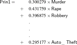
$\begin{eqnarray*} \Variable{Prin1} = & & 0.300279 \times \Variable{Murder}\\ & + & 0.431759 \times \Variable{Rape} \\ & + & 0.396875 \times \Variable{Robbery} \\ & & . \\ & & . \\ & & . \\ & + & 0.295177 \times \Variable{Auto\_ Theft} \end{eqnarray*}$

Similarly, the second principal component, Prin2, is

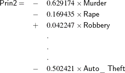
$\begin{eqnarray*} \Variable{Prin2} = & - & 0.629174 \times \Variable{Murder}\\ & - & 0.169435 \times \Variable{Rape}\\ & + & 0.042247 \times \Variable{Robbery} \\ & & . \\ & & . \\ & & . \\ & - & 0.502421 \times \Variable{Auto\_ Theft} \end{eqnarray*}$

where the variables are standardized.

Figure 91.3: Results of Principal Component Analysis: PROC PRINCOMP

Eigenvectors
	Prin1	Prin2	Prin3	Prin4	Prin5	Prin6	Prin7
Murder	0.300279	-.629174	0.178245	-.232114	0.538123	0.259117	0.267593
Rape	0.431759	-.169435	-.244198	0.062216	0.188471	-.773271	-.296485
Robbery	0.396875	0.042247	0.495861	-.557989	-.519977	-.114385	-.003903
Assault	0.396652	-.343528	-.069510	0.629804	-.506651	0.172363	0.191745
Burglary	0.440157	0.203341	-.209895	-.057555	0.101033	0.535987	-.648117
Larceny	0.357360	0.402319	-.539231	-.234890	0.030099	0.039406	0.601690
Auto_Theft	0.295177	0.502421	0.568384	0.419238	0.369753	-.057298	0.147046

The first component is a measure of the overall crime rate because the first eigenvector shows approximately equal loadings on all variables. The second eigenvector has high positive loadings on the variables Auto_Theft and Larceny and high negative loadings on the variables Murder and Assault. There is also a small positive loading on the variable Burglary and a small negative loading on the variable Rape. This component seems to measure the preponderance of property crime compared to violent crime. The interpretation of the third component is not obvious.

The ODS GRAPHICS statement enables the creation of graphs. For more information, see Chapter 21: Statistical Graphics Using ODS. The option PLOTS=SCORE(ELLIPSE NCOMP=3) in the PROC PRINCOMP statement requests the pairwise component score plots for the first three components, with a 95% prediction ellipse overlaid on each scatter plot. Figure 91.4 shows the plot of the first two components. You can identify regional trends in the plot of the first two components. Nevada and California are at the extreme right, with high overall crime rates but an average ratio of property crime to violent crime. North Dakota and South Dakota are at the extreme left, with low overall crime rates. Southeastern states tend to be at the bottom of the plot, with a higher-than-average ratio of violent crime to property crime. New England states tend to be in the upper part of the plot, with a higher-than-average ratio of property crime to violent crime. Assuming that the first two components are from a bivariate normal distribution, the ellipse identifies Nevada as a possible outlier.

Figure 91.4: Plot of the First Two Component Scores

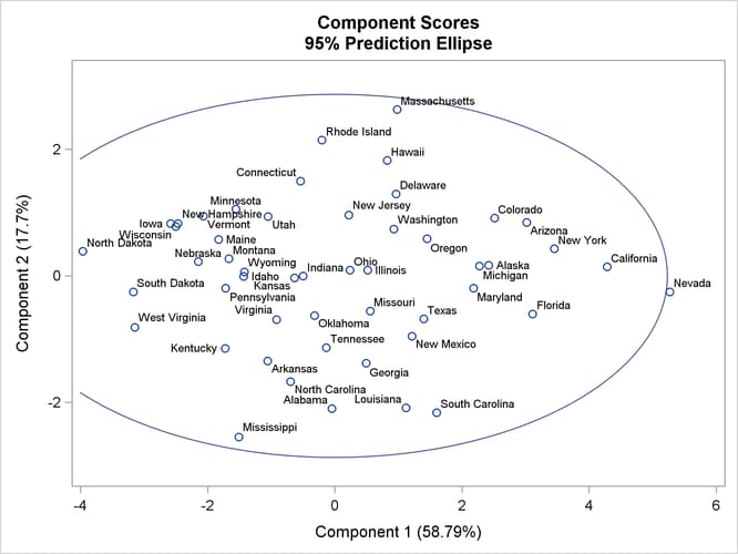
Figure 91.5 shows the plot of the first and third components. Assuming that the first and third components are from a bivariate normal distribution, the ellipse identifies Nevada, Massachusetts, and New York as possible outliers.

Figure 91.5: Plot of the First and Third Component Scores

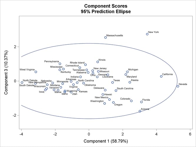
The most striking feature of the plot of the first and third principal components is that Massachusetts and New York are outliers on the third component.