Introduction to Regression Procedures
Predicted and Residual Values
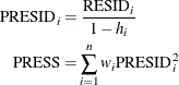
After the model has been fit, predicted and residual values are usually calculated, graphed, and output. The predicted values are calculated from the estimated regression equation; the raw residuals are calculated as the observed value minus the predicted value. Often other forms of residuals, such as studentized or cumulative residuals, are used for model diagnostics. Some procedures can calculate standard errors of residuals, predicted mean values, and individual predicted values.
Consider the ith observation, where  is the row of regressors,
  is the vector of parameter estimates, and
  is the estimate of the residual variance (the mean squared error).
The leverage value of the ith observation is defined as
is the estimate of the residual variance (the mean squared error).
The leverage value of the ith observation is defined as
![\[ h_ i = w_ i \mb{x}_ i’ (\bX ’\bW \bX )^{-1} \mb{x}_ i \]](images/statug_introreg0085.png)
where  is the design matrix for the observed data, is an arbitrary regressor vector (possibly but not necessarily a row of ),
  is a diagonal matrix of observed weights, and
  is the weight corresponding to .
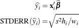
Then the predicted mean and the standard error of the predicted mean are
The standard error of the individual (future) predicted value  is
is
![\[ \mr{STDERR}(y_ i) = \sqrt {s^2 (1 + h_ i) / w_ i} \]](images/statug_introreg0088.png)
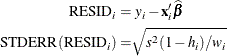
If the predictor vector  corresponds to an observation in the analysis data, then the raw residual for that observation and the standard error of
the raw residual are defined as
corresponds to an observation in the analysis data, then the raw residual for that observation and the standard error of
the raw residual are defined as
The studentized residual is the ratio of the raw residual and its estimated standard error. Symbolically,
![\[ \mr{STUDENT}_ i = \frac{\mr{RESID}_ i}{\mr{STDERR}(\mr{RESID}_ i)} \]](images/statug_introreg0091.png)
Two types of intervals provide a measure of confidence for prediction: the confidence interval for the mean value of the response, and the prediction (or forecasting) interval for an individual observation. As discussed in the section Mean Squared Error in Chapter 3: Introduction to Statistical Modeling with SAS/STAT Software, both intervals are based on the mean squared error of predicting a target based on the result of the model fit. The difference in the expressions for the confidence interval and the prediction interval occurs because the target of estimation is a constant in the case of the confidence interval (the mean of an observation) and the target is a random variable in the case of the prediction interval (a new observation).
For example, you can construct a confidence interval for the ith observation that contains the true mean value of the response with probability  . The upper and lower limits of the confidence interval for the mean value are
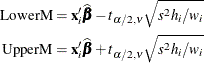
where  is the tabulated t quantile with degrees of freedom equal to the degrees of freedom for the mean squared error,
  .
.
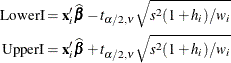
The limits for the prediction interval for an individual response are
Influential observations are those that, according to various criteria, appear to have a large influence on the analysis. One measure of influence, Cook’s D, measures the change to the estimates that results from deleting an observation,
![\[ \mr{COOKD}_ i = \frac{1}{k} \mr{STUDENT}_ i^2 \left( \frac{\mr{STDERR}(\widehat{y}_ i)}{\mr{STDERR}(\mr{RESID}_ i)} \right)^2 \]](images/statug_introreg0097.png)
where k is the number of parameters in the model (including the intercept). For more information, see Cook (1977, 1979).
The predicted residual for observation i is defined as the residual for the ith observation that results from dropping the ith observation from the parameter estimates. The sum of squares of predicted residual errors is called the PRESS statistic: