The HPCANDISC Procedure

Getting Started: HPCANDISC Procedure
The data in this example are measurements of 159 fish caught in Finland’s Lake Laengelmaevesi; this data set is available
from the Puranen. For each of the seven species (bream, roach, whitefish, parkki, perch, pike, and smelt), the weight, length, height, and
width of each fish are tallied. Three different length measurements are recorded: from the nose of the fish to the beginning
of its tail, from the nose to the notch of its tail, and from the nose to the end of its tail. The height and width are recorded
as percentages of the third length variable. The fish data set is available from the Sashelp library.
The following step uses PROC HPCANDISC to find the three canonical variables that best separate the species of fish in the
Sashelp.Fish data and create the output data set outcan. When the NCAN=3 option is specified, only the first three canonical variables are displayed. The ID statement adds the variable
Species from the input data set to the output data set. The ODS EXCLUDE statement excludes the canonical structure tables and most
of the canonical coefficient tables in order to obtain a more compact set of results. The TEMPLATE and SGRENDER procedures
create a plot of the first two canonical variables. The following statements produce Figure 50.1 through Figure 50.6:
title 'Fish Measurement Data';

proc hpcandisc data=sashelp.fish ncan=3 out=outcan;
   ods exclude tstruc bstruc pstruc tcoef pcoef;
   id Species;
   class Species;
   var Weight Length1 Length2 Length3 Height Width;
run;

proc template;
   define statgraph scatter;
      begingraph;
         entrytitle 'Fish Measurement Data';
         layout overlayequated / equatetype=fit
            xaxisopts=(label='Canonical Variable 1')
            yaxisopts=(label='Canonical Variable 2');
            scatterplot x=Can1 y=Can2 / group=species name='fish';
            layout gridded / autoalign=(topright);
               discretelegend 'fish' / border=false opaque=false;
            endlayout;
         endlayout;
      endgraph;
   end;
run;

proc sgrender data=outcan template=scatter;
run;
PROC HPCANDISC begins by displaying performance information, data access information, and summary information about the variables in the analysis, as shown in Figure 50.1.
The "Performance Information" table shows the procedure executes in single-machine mode; that is, the data reside and the computation is conducted on the machine where the SAS session executes. This run of the HPCANDISC procedure took place on a multicore machine that had four CPUs; one computational thread was spawned per CPU.
The "Data Access Information" table shows that the input data set and the output data set are both accessed with the V9 (base) engine on the client machine where the MVA SAS session executes.
The summary information includes the number of observations, the number of quantitative variables in the analysis (specified using the VAR statement), and the number of class levels in the classification variable (specified using the CLASS statement). The value and frequency of each class level are also displayed.
Figure 50.1: Fish Data: Performance, Data Access, and Summary Information
Figure 50.2 displays the "Multivariate Statistics and F Approximations" table. PROC HPCANDISC performs a one-way multivariate analysis of variance (one-way MANOVA) and provides four multivariate tests of the hypothesis that the class mean vectors are equal. These tests indicate that not all the mean vectors are equal (p < 0.0001).
Figure 50.2: Fish Data: MANOVA and Multivariate Tests
| Fish Measurement Data |
| Multivariate Statistics and F Approximations | |||||
|---|---|---|---|---|---|
| S=6 M=-0.5 N=72 | |||||
| Statistic | Value | F Value | Num DF | Den DF | Pr > F |
| Wilks' Lambda | 0.000363 | 90.71 | 36 | 643.89 | <.0001 |
| Pillai's Trace | 3.104651 | 26.99 | 36 | 906 | <.0001 |
| Hotelling-Lawley Trace | 52.057997 | 209.24 | 36 | 413.64 | <.0001 |
| Roy's Greatest Root | 39.134998 | 984.90 | 6 | 151 | <.0001 |
| NOTE: F Statistic for Roy's Greatest Root is an upper bound. | |||||
Figure 50.3 displays the "Canonical Correlations" table. The first canonical correlation is the greatest possible multiple correlation with the classes that you can achieve by using a linear combination of the quantitative variables. The first canonical correlation, displayed in the table, is 0.987463. The figure shows a likelihood ratio test of the hypothesis that the current canonical correlation and all smaller ones are zero. The first line is equivalent to Wilks’ lambda multivariate test.
Figure 50.3: Fish Data: Canonical Correlations
| Fish Measurement Data |
| Canonical Correlation |
Adjusted Canonical Correlation |
Approximate Standard Error |
Squared Canonical Correlation |
Eigenvalues of Inv(E)*H = CanRsq/(1-CanRsq) |
Test of H0: The canonical correlations in the current row and all that follow are zero | ||||||||
|---|---|---|---|---|---|---|---|---|---|---|---|---|---|
| Eigenvalue | Difference | Proportion | Cumulative | Likelihood Ratio |
Approximate F Value |
Num DF | Den DF | Pr > F | |||||
| 1 | 0.987463 | 0.986671 | 0.001989 | 0.975084 | 39.1350 | 29.3859 | 0.7518 | 0.7518 | 0.00036325 | 90.71 | 36 | 643.89 | <.0001 |
| 2 | 0.952349 | 0.950095 | 0.007425 | 0.906969 | 9.7491 | 7.3786 | 0.1873 | 0.9390 | 0.01457896 | 46.46 | 25 | 547.58 | <.0001 |
| 3 | 0.838637 | 0.832518 | 0.023678 | 0.703313 | 2.3706 | 1.7016 | 0.0455 | 0.9846 | 0.15671134 | 23.61 | 16 | 452.79 | <.0001 |
| 4 | 0.633094 | 0.623649 | 0.047821 | 0.400809 | 0.6689 | 0.5346 | 0.0128 | 0.9974 | 0.52820347 | 12.09 | 9 | 362.78 | <.0001 |
| 5 | 0.344157 | 0.334170 | 0.070356 | 0.118444 | 0.1344 | 0.1343 | 0.0026 | 1.0000 | 0.88152702 | 4.88 | 4 | 300 | 0.0008 |
| 6 | 0.005701 | . | 0.079806 | 0.000033 | 0.0000 | 0.0000 | 1.0000 | 0.99996749 | 0.00 | 1 | 151 | 0.9442 | |
Figure 50.4 displays the "Raw Canonical Coefficients" table. The first canonical variable, Can1, shows that the linear combination of the centered variables Can1 = –0.0006 
Weight – 0.33 Length1 2.49 Length2 + 2.60 Length3 + 1.12 Height – 1.45 Width separates the species most effectively.
Figure 50.4: Fish Data: Raw Canonical Coefficients
Figure 50.5 displays the "Class Means on Canonical Variables" table. PROC HPCANDISC computes the means of the canonical variables for
each class. The first canonical variable is the linear combination of the variables Weight, Length1, Length2, Length3, Height, and Width that provides the greatest difference (in terms of a univariate F test) between the class means. The second canonical variable provides the greatest difference between class means while being
uncorrelated with the first canonical variable.
Figure 50.5: Fish Data: Class Means for Canonical Variables
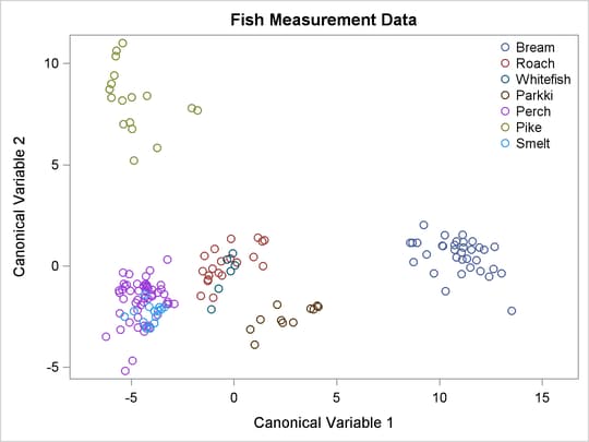
Figure 50.6 displays a plot of the first two canonical variables, which shows that Can1 discriminates among three groups: (1) bream; (2) whitefish, roach, and parkki; and (3) smelt, pike, and perch. Can2 best discriminates between pike and the other species.
Figure 50.6: Fish Data: Plot of First Two Canonical Variables