The HPCANDISC Procedure

Example 50.1 Analyzing Iris Data with PROC HPCANDISC
The iris data that were published by Fisher (1936) have been widely used for examples in discriminant analysis and cluster analysis. The sepal length, sepal width, petal length,
and petal width are measured in millimeters in 50 iris specimens from each of three species: Iris setosa, I. versicolor, and I. virginica. The iris data set is available from the Sashelp library.
This example is a canonical discriminant analysis that creates an output data set that contains scores on the canonical variables
and plots the canonical variables. The ID statement is specified to add the variable Species from the input data set to the output data set.
The following statements produce Output 50.1.1 through Output 50.1.6:
title 'Fisher (1936) Iris Data';

proc hpcandisc data=sashelp.iris out=outcan distance anova;
   id Species;
   class Species;
   var SepalLength SepalWidth PetalLength PetalWidth;
run;
Output 50.1.1 displays performance information, data access information, and summary information about the observations and the classes in the data set.
Output 50.1.1: Iris Data: Performance, Data Access, and Summary Information
Output 50.1.2 shows results from the DISTANCE option in the PROC HPCANDISC statement, which display squared Mahalanobis distances between class means.
Output 50.1.2: Iris Data: Squared Mahalanobis Distances and Distance Statistics
Output 50.1.3 displays univariate and multivariate statistics. The ANOVA option uses univariate statistics to test the hypothesis that
the class means are equal. The resulting R-square values range from 0.4008 for SepalWidth to 0.9414 for PetalLength, and each variable is significant at the 0.0001 level. The multivariate test for differences between the class levels (which
is displayed by default) is also significant at the 0.0001 level; you would expect this from the highly significant univariate
test results.
Output 50.1.3: Iris Data: Univariate and Multivariate Statistics
| Fisher (1936) Iris Data |
| Univariate Test Statistics | ||||||||
|---|---|---|---|---|---|---|---|---|
| F Statistics, Num DF=2, Den DF=147 | ||||||||
| Variable | Label | Total Standard Deviation |
Pooled Standard Deviation |
Between Standard Deviation |
R-Square | R-Square / (1-Rsq) |
F Value | Pr > F |
| SepalLength | Sepal Length (mm) | 8.28066 | 5.14789 | 7.95061 | 0.6187 | 1.6226 | 119.26 | <.0001 |
| SepalWidth | Sepal Width (mm) | 4.35866 | 3.39688 | 3.36822 | 0.4008 | 0.6688 | 49.16 | <.0001 |
| PetalLength | Petal Length (mm) | 17.65298 | 4.30334 | 20.90700 | 0.9414 | 16.0566 | 1180.16 | <.0001 |
| PetalWidth | Petal Width (mm) | 7.62238 | 2.04650 | 8.96735 | 0.9289 | 13.0613 | 960.01 | <.0001 |
| Multivariate Statistics and F Approximations | |||||
|---|---|---|---|---|---|
| S=2 M=0.5 N=71 | |||||
| Statistic | Value | F Value | Num DF | Den DF | Pr > F |
| Wilks' Lambda | 0.023439 | 199.15 | 8 | 288 | <.0001 |
| Pillai's Trace | 1.191899 | 53.47 | 8 | 290 | <.0001 |
| Hotelling-Lawley Trace | 32.477320 | 582.20 | 8 | 203.4 | <.0001 |
| Roy's Greatest Root | 32.191929 | 1166.96 | 4 | 145 | <.0001 |
| NOTE: F Statistic for Roy's Greatest Root is an upper bound. | |||||
| NOTE: F Statistic for Wilks' Lambda is exact. | |||||
Output 50.1.4 displays canonical correlations and eigenvalues. The R square between Can1 and the class variable, 0.969872, is much larger than the corresponding R square for Can2, 0.222027.
Output 50.1.4: Iris Data: Canonical Correlations and Eigenvalues
| Fisher (1936) Iris Data |
| Canonical Correlation |
Adjusted Canonical Correlation |
Approximate Standard Error |
Squared Canonical Correlation |
Eigenvalues of Inv(E)*H = CanRsq/(1-CanRsq) |
Test of H0: The canonical correlations in the current row and all that follow are zero | ||||||||
|---|---|---|---|---|---|---|---|---|---|---|---|---|---|
| Eigenvalue | Difference | Proportion | Cumulative | Likelihood Ratio |
Approximate F Value |
Num DF | Den DF | Pr > F | |||||
| 1 | 0.984821 | 0.984508 | 0.002468 | 0.969872 | 32.1919 | 31.9065 | 0.9912 | 0.9912 | 0.02343863 | 199.15 | 8 | 288 | <.0001 |
| 2 | 0.471197 | 0.461445 | 0.063734 | 0.222027 | 0.2854 | 0.0088 | 1.0000 | 0.77797337 | 13.79 | 3 | 145 | <.0001 | |
Output 50.1.5 displays correlations between canonical and original variables.
Output 50.1.5: Iris Data: Correlations between Canonical and Original Variables
Output 50.1.6 displays canonical coefficients. The raw canonical coefficients for the first canonical variable, Can1, show that the class levels differ most widely on the linear combination of the centered variables:  .
.
Output 50.1.6: Iris Data: Canonical Coefficients
| Fisher (1936) Iris Data |
| Total-Sample Standardized Canonical Coefficients | |||
|---|---|---|---|
| Variable | Label | Can1 | Can2 |
| SepalLength | Sepal Length (mm) | -0.68678 | 0.01996 |
| SepalWidth | Sepal Width (mm) | -0.66883 | 0.94344 |
| PetalLength | Petal Length (mm) | 3.88580 | -1.64512 |
| PetalWidth | Petal Width (mm) | 2.14224 | 2.16414 |
Output 50.1.7 displays class means on canonical variables.
Output 50.1.7: Iris Data: Canonical Means
The TEMPLATE and SGRENDER procedures are used to create a plot of the first two canonical variables. The following statements produce Output 50.1.8:
proc template;
   define statgraph scatter;
      begingraph;
         entrytitle 'Fisher (1936) Iris Data';
         layout overlayequated / equatetype=fit
            xaxisopts=(label='Canonical Variable 1')
            yaxisopts=(label='Canonical Variable 2');
            scatterplot x=Can1 y=Can2 / group=species name='iris';
            layout gridded / autoalign=(topleft);
               discretelegend 'iris' / border=false opaque=false;
            endlayout;
         endlayout;
      endgraph;
   end;
run;

proc sgrender data=outcan template=scatter;
run;
Output 50.1.8: Iris Data: Plot of First Two Canonical Variables
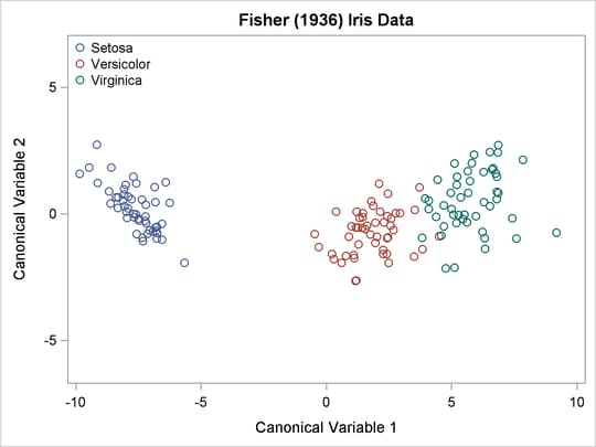
The plot of canonical variables in Output 50.1.8 shows that of the two canonical variables, Can1 has more discriminatory power.