The FACTOR Procedure
-
Overview

- Getting Started
-
Syntax
-
DetailsInput Data SetOutput Data SetsConfidence Intervals and the Salience of Factor LoadingsSimplicity Functions for RotationsMissing ValuesCautionsFactor ScoresVariable Weights and Variance ExplainedHeywood Cases and Other Anomalies about Communality EstimatesTime RequirementsDisplayed OutputODS Table NamesODS Graphics
-
Examples
- References
Example 37.5 Creating Path Diagrams for Factor Solutions
The section Getting Started: FACTOR Procedure analyzes a data set that contains 14 ratings of 103 police officers to demonstrate some basic techniques in factor analysis. To illustrate the creation and uses of path diagrams, this example analyzes this data set again by using the following statements:
ods graphics on;

proc factor data=jobratings(drop='Overall Rating'n)
   priors=smc rotate=quartimin plots=pathdiagram;
label
   'Judgment under Pressure'n ='Judgment'
   'Communication Skills'n = 'Comm Skills'
   'Interpersonal Sensitivity'n = 'Sensitivity'
   'Willingness to Confront Problems'n = 'Confront Problems'
   'Desire for Self-Improvement'n = 'Self-Improve'
   'Observational Skills'n = 'Obs Skills'
   'Dependability'n = 'Dependable';
run;
The PRIORS=SMC option specifies that the squared multiple correlations are to be used as the prior communality estimates. As a result, the factors are extracted by the principal factor method. The ROTATE=QUARTIMIN option requests the use of the quartimin rotation to obtain the final factor solution. The PLOTS=PATHDIAGRAM option requests a path diagram for the final solution. The LABEL statement specifies labels for variables.
When variables do not have labels, PROC FACTOR displays the variable names in path diagrams. But when variables have labels, PROC FACTOR displays labels, instead of variable names, in path diagrams. Because some variables in this example have very long variables names, PROC FACTOR might truncate these long names in the output path diagram. Therefore, to avoid truncations in the output diagram, you can either create a data set with shorter variable names or use the LABEL statement to specify shorter labels. This example illustrates the use of the LABEL statement.
Except for the PLOTS=PATHDIAGRAM option, previous examples have already described the FACTOR options that are used in this example. Therefore, this example focuses only on the creation of path diagrams.
Output 37.5.1 and Output 37.5.2 show the quartimin-rotated factor correlations and factor pattern, respectively.
Output 37.5.1: Quartimin-Rotated Factor Correlations
Output 37.5.2: Quartimin-Rotated Factor Pattern
| Rotated Factor Pattern (Standardized Regression Coefficients) | ||||
|---|---|---|---|---|
| Factor1 | Factor2 | Factor3 | ||
| Communication Skills | Comm Skills | 0.21280 | 0.13541 | 0.61091 |
| Problem Solving | 0.17222 | 0.01424 | 0.68767 | |
| Learning Ability | -0.09904 | 0.24961 | 0.65430 | |
| Judgment under Pressure | Judgment | 0.49876 | -0.02005 | 0.48879 |
| Observational Skills | Obs Skills | -0.15748 | 0.67661 | 0.30273 |
| Willingness to Confront Problems | Confront Problems | -0.19106 | 0.66639 | 0.31135 |
| Interest in People | 0.84249 | 0.12734 | -0.00710 | |
| Interpersonal Sensitivity | Sensitivity | 0.87832 | -0.12964 | 0.15116 |
| Desire for Self-Improvement | Self-Improve | 0.19078 | 0.49891 | 0.23297 |
| Appearance | 0.05254 | 0.53846 | 0.10857 | |
| Dependability | Dependable | 0.39241 | 0.50035 | 0.12032 |
| Physical Ability | 0.14404 | 0.63901 | -0.15220 | |
| Integrity | 0.68277 | 0.32719 | -0.01887 | |
Output 37.5.3 shows the path diagram for the quartimin-rotated factor solution. The path diagram represents correlations among factors
by double-headed links or paths. For example, Output 37.5.3 represents the correlation between Factor1 and Factor2 by a curved doubled-headed link. The numerical value, 0.36, is the correlation between the two factors, as can be verified
from the table in Output 37.5.1. Similarly, Output 37.5.3 shows other factor correlations by curved doubled-headed links.
Output 37.5.3: Default Path Diagram for the Quartimin-Rotated Solution
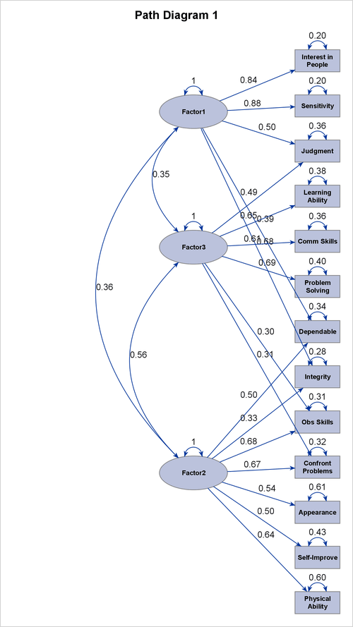
The path diagram in Output 37.5.3 also represents factor variances and error variances by double-headed links. However, each of these links points to an individual variable, rather than to a pair of variables as the double-headed links for correlations do. The path diagram also displays the numerical values of factor variances or error variances next to the associated links.
The directed links from factors to variables in the path diagram represent the effects of factors on the variables. The path
diagram displays the numerical values of these effects, which are the loading estimates that are shown in Output 37.5.2. However, to aid the interpretation of the factors, the path diagram does not show all factor loadings or their corresponding
links. By default, the path diagram displays only the links that have loadings greater than 0.3 in magnitude. For example,
instead of associating Factor1 with all variables, the path diagram in Output 37.5.3 displays only five directed links from Factor1 to the variables. The weaker links that have loadings less than 0.3 are not shown.
The use of the 0.3 loading value (or greater in magnitude) for relating factors to variables is referred to as the "0.3-rule"
in the field of factor analysis. However, this is only a convention, and sometimes you might want to use a different criterion
to interpret the factors. For example, the path diagram in Output 37.5.3 shows that variables Dependability, Integrity, and Observational Skills are all associated with more than one factor. Hence, factors might not be interpreted unambiguously.
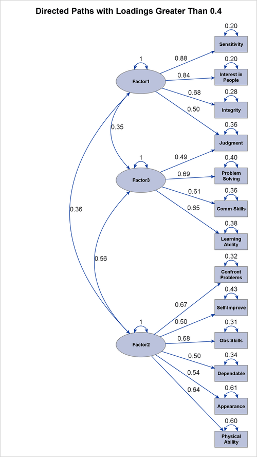
One way to tackle this interpretation problem is to set a stricter criterion for interpreting factors. You can use the FUZZ= option to set such a criterion. For example, you specify the following PATHDIAGRAM statement to display only the strong directed links that are associated with a 0.4 or greater magnitude in the loading estimates:
pathdiagram fuzz=0.4 title='Directed Paths with Loadings Greater Than 0.4';
The preceding statement also uses the TITLE= option to specify a customized title for the path diagram. Output 37.5.4 shows the resulting path diagram. In this path diagram, only one observed variable is linked to two factors. All other observed variables link to unique factors. Therefore, compared to the path diagram in Output 37.5.3, the path diagram in Output 37.5.4 provides a much "cleaner" picture for interpreting the factors.
Output 37.5.4: Path Diagram Showing Strong Links
The current example has 13 observed variables in the path diagram. By default, PROC FACTOR uses the process-flow algorithm to lay out the variables. However, when the number of observed variables becomes large, the process-flow algorithm needs a lot of vertical space to align all observed variables in a vertical line. Displaying such a "long" path diagram in limited space (for example, in a page) might compromise the clarity of the path diagram.
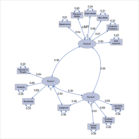
To handle this issue, PROC FACTOR switches to the GRIP algorithm when the number of variables is greater than 14. However, you can override the layout algorithm whenever you find it useful to do so. For example, the ARRANGE=GRIP option in the following PATHDIAGRAM statement requests that the GRIP algorithm be used:
pathdiagram fuzz=0.4 arrange=grip scale=0.85 notitle;
The SCALE= option shrinks the nodes so that the nodes are well-separated in the path diagram. If you do not use this option, some nodes would have been overlapped. The NOTITLE option suppresses the display of the title. Output 37.5.5 shows the resulting path diagram, which spreads out the variables instead of aligning them vertically, as it does when it uses the process-flow algorithm in Output 37.5.4.
Output 37.5.5: Path Diagram Showing Strong Links by Using the ARRANGE=GRIP Algorithm
For more information about the options for customizing path diagrams, see the PATHDIAGRAM statement.