The DISCRIM Procedure

Background
The following notation is used to describe the classification methods:

-
a p-dimensional vector containing the quantitative variables of an observation

-
the pooled covariance matrix
- t
-
a subscript to distinguish the groups

-
the number of training set observations in group t

-
the p-dimensional vector containing variable means in group t

-
the covariance matrix within group t

-
the determinant of

-
the prior probability of membership in group t

-
the posterior probability of an observation
belonging to group t

-
the probability density function for group t

-
the group-specific density estimate at
from group t

-
 , the estimated unconditional density at

-
the classification error rate for group t
Bayes’ Theorem
Assuming that the prior probabilities of group membership are known and that the group-specific densities at can be estimated, PROC DISCRIM computes , the probability of belonging to group t, by applying Bayes’ theorem:
![\[ p(t|\mb{x}) = \frac{q_ t f_ t(\mb{x})}{f(\mb{x})} \]](images/statug_discrim0024.png)
PROC DISCRIM partitions a p-dimensional vector space into regions  , where the region is the subspace containing all p-dimensional vectors
  such that
  is the largest among all groups. An observation is classified as coming from group t if it lies in region .
Parametric Methods
Assuming that each group has a multivariate normal distribution, PROC DISCRIM develops a discriminant function or classification criterion by using a measure of generalized squared distance. The classification criterion is based on either the individual within-group covariance matrices or the pooled covariance matrix; it also takes into account the prior probabilities of the classes. Each observation is placed in the class from which it has the smallest generalized squared distance. PROC DISCRIM also computes the posterior probability of an observation belonging to each class.
The squared Mahalanobis distance from to group t is
![\[ d_ t^2(\mb{x}) = (\mb{x} - \mb{m}_ t)^{\prime } \mb{V}_ t^{-1}(\mb{x} - \mb{m}_ t) \]](images/statug_discrim0027.png)
where  if the within-group covariance matrices are used, or
  if the pooled covariance matrix is used.
The group-specific density estimate at
from group t is then given by
![\[ f_ t(\mb{x}) = (2 \pi )^{-\frac{p}{2}} |\mb{V}_ t|^{-\frac{1}{2}} \exp \left(-0.5 d_ t^2(\mb{x}) \right) \]](images/statug_discrim0030.png)
Using Bayes’ theorem, the posterior probability of belonging to group t is
![\[ p(t|\mb{x}) = \frac{q_ t f_ t(\mb{x})}{\sum _ u q_ u f_ u(\mb{x})} \]](images/statug_discrim0031.png)
where the summation is over all groups.
The generalized squared distance from
to group t is defined as
![\[ D_ t^2(\mb{x}) = d_ t^2(\mb{x}) + g_1(t) + g_2(t) \]](images/statug_discrim0032.png)
where

and

The posterior probability of belonging to group t is then equal to
![\[ p(t|\mb{x}) = \frac{ \exp \left(-0.5 D_ t^2(\mb{x}) \right)}{\sum _ u \exp \left( -0.5 D_ u^2(\mb{x}) \right) } \]](images/statug_discrim0035.png)
The discriminant scores are  . An observation is classified into group u if setting t = u produces the largest value of or the smallest value of
  . If this largest posterior probability is less than the threshold specified, is labeled as
 Other.
Nonparametric Methods
Nonparametric discriminant methods are based on nonparametric estimates of group-specific probability densities. Either a kernel method or the k-nearest-neighbor method can be used to generate a nonparametric density estimate in each group and to produce a classification criterion. The kernel method uses uniform, normal, Epanechnikov, biweight, or triweight kernels in the density estimation.
Either Mahalanobis distance or Euclidean distance can be used to determine proximity. When the k-nearest-neighbor method is used, the Mahalanobis distances are based on the pooled covariance matrix. When a kernel method is used, the Mahalanobis distances are based on either the individual within-group covariance matrices or the pooled covariance matrix. Either the full covariance matrix or the diagonal matrix of variances can be used to calculate the Mahalanobis distances.
The squared distance between two observation vectors, and , in group t is given by
![\[ d_ t^2(\mb{x},\mb{y}) = (\mb{x}-\mb{y})^{\prime } \mb{V}_ t^{-1} (\mb{x}-\mb{y}) \]](images/statug_discrim0038.png)
where  has one of the following forms:
![\[ \mb{V}_ t = \left\{ \begin{array}{lcl} \mb{S}_ p & & \mbox{the pooled covariance matrix} \\ \mbox{diag}(\mb{S}_ p) & & \mbox{the diagonal matrix of the pooled covariance matrix} \\ \mb{S}_ t & & \mbox{the covariance matrix within group } t \\ \mbox{diag}(\mb{S}_ t) & & \mbox{the diagonal matrix of the covariance matrix within group } t \\ \mb{I} & & \mbox{the identity matrix} \\ \end{array} \right. \]](images/statug_discrim0039.png)
The classification of an observation vector is based on the estimated group-specific densities from the training set. From these estimated densities, the posterior probabilities
of group membership at are evaluated. An observation is classified into group u if setting  produces the largest value of . If there is a tie for the largest probability or if this largest probability is less than the threshold specified, is labeled as
 Other.
The kernel method uses a fixed radius, r, and a specified kernel,  , to estimate the group t density at each observation vector . Let
  be a p-dimensional vector. Then the volume of a p-dimensional unit sphere bounded by
  is
is
![\[ v_0 = \frac{ \pi ^{\frac{p}{2}}}{ \Gamma \left( \frac{p}{2} + 1 \right) } \]](images/statug_discrim0044.png)
where  represents the gamma function (see
SAS Functions and CALL Routines: Reference).
represents the gamma function (see
SAS Functions and CALL Routines: Reference).
Thus, in group t, the volume of a p-dimensional ellipsoid bounded by  is
is
![\[ v_ r(t) = r^ p |\mb{V}_ t|^{\frac{1}{2}} v_0 \]](images/statug_discrim0047.png)
The kernel method uses one of the following densities as the kernel density in group t:
![\[ K_ t(\mb{z}) = \left\{ \begin{array}{lcl} \displaystyle \frac{1}{v_ r(t)} & & \mbox{if } \mb{z}^{\prime } \mb{V}_ t^{-1} \mb{z} \leq r^2 \\ 0 & & \mbox{elsewhere} \\ \end{array} \right. \]](images/statug_discrim0048.png)
Normal Kernel (with mean zero, variance  )
)
![\[ K_ t(\mb{z}) = \frac{1}{c_0(t)} \exp \left(-\frac{1}{2r^2} \mb{z}^{\prime } \mb{V}_ t^{-1} \mb{z} \right) \]](images/statug_discrim0049.png)
where  .
.
![\[ K_ t(\mb{z}) = \left\{ \begin{array}{lcl} \displaystyle c_1(t) \left( 1 - \frac{1}{r^2}\mb{z}^{\prime } \mb{V}_ t^{-1} \mb{z} \right) & & \mbox{if } \mb{z}^{\prime } \mb{V}_ t^{-1} \mb{z} \leq r^2 \\ 0 & & \mbox{elsewhere} \\ \end{array} \right. \]](images/statug_discrim0051.png)
where  .
.
![\[ K_ t(\mb{z}) = \left\{ \begin{array}{lcl} \displaystyle c_2(t) \left( 1 - \frac{1}{r^2}\mb{z}^{\prime } \mb{V}_ t^{-1} \mb{z} \right)^2 & & \mbox{if } \mb{z}^{\prime } \mb{V}_ t^{-1} \mb{z} \leq r^2 \\ 0 & & \mbox{elsewhere} \\ \end{array} \right. \]](images/statug_discrim0053.png)
where  .
.
![\[ K_ t(\mb{z}) = \left\{ \begin{array}{lcl} \displaystyle c_3(t) \left( 1 - \frac{1}{r^2}\mb{z}^{\prime } \mb{V}_ t^{-1} \mb{z} \right)^3 & & \mbox{if } \mb{z}^{\prime } \mb{V}_ t^{-1} \mb{z} \leq r^2 \\ 0 & & \mbox{elsewhere} \\ \end{array} \right. \]](images/statug_discrim0055.png)
where  .
.
The group t density at is estimated by
![\[ f_ t(\mb{x}) = \frac{1}{n_ t} \sum _\mb {y} K_ t(\mb{x}-\mb{y}) \]](images/statug_discrim0057.png)
where the summation is over all observations in group t, and is the specified kernel function. The posterior probability of membership in group t is then given by
where  is the estimated unconditional density. If is zero, the observation is labeled as
 Other.
The uniform-kernel method treats  as a multivariate uniform function with density uniformly distributed over
  . Let
. Let  be the number of training set observations from group t within the closed ellipsoid centered at specified by
  . Then the group t density at is estimated by
![\[ f_ t(\mb{x}) = \frac{k_ t}{n_ t v_ r(t)} \]](images/statug_discrim0062.png)
When the identity matrix or the pooled within-group covariance matrix is used in calculating the squared distance,  is a constant, independent of group membership. The posterior probability of belonging to group t is then given by
![\[ p(t|\mb{x}) = \frac{\frac{\displaystyle q_ t k_ t}{\displaystyle n_ t}}{\sum _ u \frac{\displaystyle q_ u k_ u}{\displaystyle n_ u}} \]](images/statug_discrim0064.png)
If the closed ellipsoid centered at does not include any training set observations, is zero and is labeled as Other. When the prior probabilities are equal, is proportional to  and is classified into the group that has the highest proportion of observations in the closed ellipsoid. When the prior probabilities
are proportional to the group sizes,
and is classified into the group that has the highest proportion of observations in the closed ellipsoid. When the prior probabilities
are proportional to the group sizes,  , is classified into the group that has the largest number of observations in the closed ellipsoid.
The nearest-neighbor method fixes the number, k, of training set points for each observation . The method finds the radius  that is the distance from to the kth-nearest training set point in the metric
  . Consider a closed ellipsoid centered at bounded by
  ; the nearest-neighbor method is equivalent to the uniform-kernel method with a location-dependent radius . Note that, with ties, more than k training set points might be in the ellipsoid.
Using the k-nearest-neighbor rule, the  (or more with ties) smallest distances are saved. Of these k distances, let represent the number of distances that are associated with group t. Then, as in the uniform-kernel method, the estimated group t density at is
![\[ f_ t(\mb{x}) = \frac{k_ t}{n_ t v_ k(\mb{x})} \]](images/statug_discrim0071.png)
where  is the volume of the ellipsoid bounded by
  . Since the pooled within-group covariance matrix is used to calculate the distances used in the nearest-neighbor method,
the volume is a constant independent of group membership. When k = 1 is used in the nearest-neighbor rule, is classified into the group associated with the point that yields the smallest squared distance
. Since the pooled within-group covariance matrix is used to calculate the distances used in the nearest-neighbor method,
the volume is a constant independent of group membership. When k = 1 is used in the nearest-neighbor rule, is classified into the group associated with the point that yields the smallest squared distance  . Prior probabilities affect nearest-neighbor results in the same way that they affect uniform-kernel results.
With a specified squared distance formula (METRIC=, POOL=), the values of r and k determine the degree of irregularity in the estimate of the density function, and they are called smoothing parameters. Small values of r or k produce jagged density estimates, and large values of r or k produce smoother density estimates. Various methods for choosing the smoothing parameters have been suggested, and there is as yet no simple solution to this problem.
For a fixed kernel shape, one way to choose the smoothing parameter r is to plot estimated densities with different values of r and to choose the estimate that is most in accordance with the prior information about the density. For many applications, this approach is satisfactory.
Another way of selecting the smoothing parameter r
is to choose a value that optimizes a given criterion. Different groups might have different sets of optimal values. Assume
that the unknown density has bounded and continuous second derivatives and that the kernel is a symmetric probability density
function. One criterion is to minimize an approximate mean integrated square error of the estimated density (Rosenblatt 1956). The resulting optimal value of r depends on the density function and the kernel. A reasonable choice for the smoothing parameter r is to optimize the criterion with the assumption that group t has a normal distribution with covariance matrix . Then, in group t, the resulting optimal value for r is given by
![\[ \left( \frac{A(K_ t)}{n_ t} \right)^{1/(p+4)} \]](images/statug_discrim0075.png)
where the optimal constant  depends on the kernel (Epanechnikov 1969). For some useful kernels, the constants are given by the following:
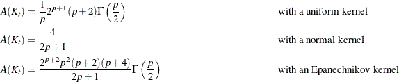
These selections of are derived under the assumption that the data in each group are from a multivariate normal distribution with covariance
matrix . However, when the Euclidean distances are used in calculating the squared distance  , the smoothing constant should be multiplied by s, where s is an estimate of standard deviations for all variables. A reasonable choice for s is
![\[ s = \left( \frac{1}{p} \sum s_{jj} \right)^{\frac{1}{2}} \]](images/statug_discrim0079.png)
where  are group t marginal variances.
The DISCRIM procedure uses only a single smoothing parameter for all groups. However, the selection of the matrix in the distance
formula (from the METRIC= or POOL= option), enables individual groups and variables to have different scalings. When , the matrix used in calculating the squared distances, is an identity matrix, the kernel estimate at each data point is scaled
equally for all variables in all groups. When is the diagonal matrix of a covariance matrix, each variable in group t is scaled separately by its variance in the kernel estimation, where the variance can be the pooled variance  or an individual within-group variance
  . When is a full covariance matrix, the variables in group t are scaled simultaneously by in the kernel estimation.
In nearest-neighbor methods, the choice of k is usually relatively uncritical (Hand 1982). A practical approach is to try several different values of the smoothing parameters within the context of the particular application and to choose the one that gives the best cross validated estimate of the error rate.
Classification Error-Rate Estimates
A classification criterion can be evaluated by its performance in the classification of future observations. PROC DISCRIM uses two types of error-rate estimates to evaluate the derived classification criterion based on parameters estimated by the training sample:
-
error-count estimates
-
posterior probability error-rate estimates
The error-count estimate is calculated by applying the classification criterion derived from the training sample to a test set and then counting the number of misclassified observations. The group-specific error-count estimate is the proportion of misclassified observations in the group. When the test set is independent of the training sample, the estimate is unbiased. However, the estimate can have a large variance, especially if the test set is small.
When the input data set is an ordinary SAS data set and no independent test sets are available, the same data set can be used both to define and to evaluate the classification criterion. The resulting error-count estimate has an optimistic bias and is called an apparent error rate. To reduce the bias, you can split the data into two sets—one set for deriving the discriminant function and the other set for estimating the error rate. Such a split-sample method has the unfortunate effect of reducing the effective sample size.
Another way to reduce bias is cross validation (Lachenbruch and Mickey 1968). Cross validation treats n – 1 out of n training observations as a training set. It determines the discriminant functions based on these n – 1 observations and then applies them to classify the one observation left out. This is done for each of the n training observations. The misclassification rate for each group is the proportion of sample observations in that group that are misclassified. This method achieves a nearly unbiased estimate but with a relatively large variance.
To reduce the variance in an error-count estimate, smoothed error-rate estimates are suggested (Glick 1978). Instead of summing terms that are either zero or one as in the error-count estimator, the smoothed estimator uses a continuum of values between zero and one in the terms that are summed. The resulting estimator has a smaller variance than the error-count estimate. The posterior probability error-rate estimates provided by the POSTERR option in the PROC DISCRIM statement (see the section Posterior Probability Error-Rate Estimates) are smoothed error-rate estimates. The posterior probability estimates for each group are based on the posterior probabilities of the observations classified into that same group. The posterior probability estimates provide good estimates of the error rate when the posterior probabilities are accurate. When a parametric classification criterion (linear or quadratic discriminant function) is derived from a nonnormal population, the resulting posterior probability error-rate estimators might not be appropriate.
The overall error rate is estimated through a weighted average of the individual group-specific error-rate estimates, where the prior probabilities are used as the weights.
To reduce both the bias and the variance of the estimator, Hora and Wilcox (1982) compute the posterior probability estimates based on cross validation. The resulting estimates are intended to have both low variance from using the posterior probability estimate and low bias from cross validation. They use Monte Carlo studies on two-group multivariate normal distributions to compare the cross validation posterior probability estimates with three other estimators: the apparent error rate, cross validation estimator, and posterior probability estimator. They conclude that the cross validation posterior probability estimator has a lower mean squared error in their simulations.
Quasi-inverse
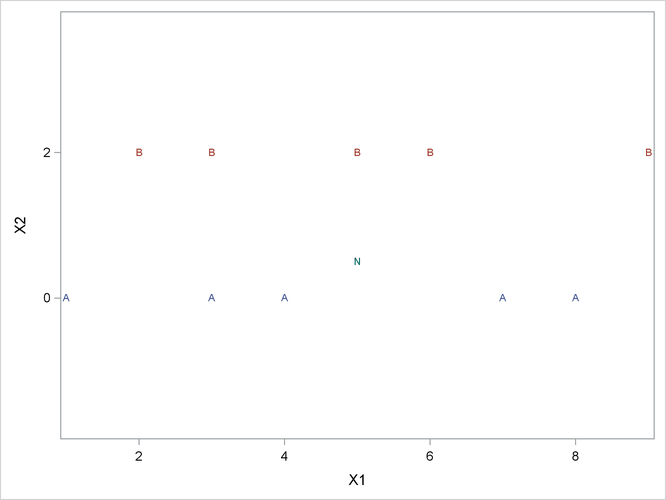
Consider the plot shown in Figure 35.6 with two variables, X1 and X2, and two classes, A and B. The within-class covariance matrix is diagonal, with a positive value for X1 but zero for X2. Using a Moore-Penrose pseudo-inverse would effectively ignore X2 in doing the classification, and the two classes would have a zero generalized distance and could not be discriminated at
all. The quasi inverse used by PROC DISCRIM replaces the zero variance for X2 with a small positive number to remove the singularity. This permits X2 to be used in the discrimination and results correctly in a large generalized distance between the two classes and a zero
error rate. It also permits new observations, such as the one indicated by N, to be classified in a reasonable way. PROC CANDISC
also uses a quasi inverse when the total-sample covariance matrix is considered to be singular and Mahalanobis distances are
requested. This problem with singular within-class covariance matrices is discussed in Ripley (1996, p. 38). The use of the quasi inverse is an innovation introduced by SAS.
Figure 35.6: Plot of Data with Singular Within-Class Covariance Matrix
Let  be a singular covariance matrix. The matrix can be either a within-group covariance matrix, a pooled covariance matrix, or a total-sample covariance matrix. Let v be the number of variables in the VAR statement, and let the nullity n be the number of variables among them with (partial) R square exceeding 1 – p. If the determinant of (Testing of Homogeneity of Within Covariance Matrices) or the inverse of (Squared Distances and Generalized Squared Distances) is required, a quasi determinant or quasi inverse is used instead.
With raw data input, PROC DISCRIM scales each variable to unit total-sample variance before calculating this quasi inverse.
The calculation is based on the spectral decomposition
be a singular covariance matrix. The matrix can be either a within-group covariance matrix, a pooled covariance matrix, or a total-sample covariance matrix. Let v be the number of variables in the VAR statement, and let the nullity n be the number of variables among them with (partial) R square exceeding 1 – p. If the determinant of (Testing of Homogeneity of Within Covariance Matrices) or the inverse of (Squared Distances and Generalized Squared Distances) is required, a quasi determinant or quasi inverse is used instead.
With raw data input, PROC DISCRIM scales each variable to unit total-sample variance before calculating this quasi inverse.
The calculation is based on the spectral decomposition  , where
  is a diagonal matrix of eigenvalues
  ,
,  , where
  when
when  , and
, and  is a matrix with the corresponding orthonormal eigenvectors of as columns. When the nullity n is less than v, set
  for
for  , and
, and  for
for  , where
![\[ \bar{\lambda } = \frac{1}{v-n} \sum _{k=1}^{v-n} \lambda _ k \]](images/statug_discrim0094.png)
When the nullity n is equal to v, set  , for
, for  . A quasi determinant is then defined as the product of
  ,
,  . Similarly, a quasi inverse is then defined as
  , where
  is a diagonal matrix of values
  .
.