The IRT Procedure

The data set in this example comes from the 1978 Quality of American Life Survey. The survey was administered to a sample of US residents aged 18 years and older in 1978. Subjects were asked to rate their satisfaction with many different aspects of their lives. This example includes 14 items. Some of the items are as follows:
-
satisfaction with community
-
satisfaction with neighbors
-
satisfaction with amount of education received
-
satisfaction with health
-
satisfaction with job
-
satisfaction with income
Originally these items were designed with seven-point scales, where 1 indicates most unsatisfied and 7 indicates most satisfied.
For illustration purposes, these items have been reorganized into a different number of categories, which ranges from 2 to
7. This example uses 1,000 random samples from the original data set. The following DATA step creates the data set IrtQls:
data IrtQls;
   input item1-item14 @@;
   datalines;
 1   1   2   1   1    2    2    2    .    2    2    2    2    2
 2   2   2   2   2    3    4    1    .    2    5    6    4    4

   ... more lines ...

 1   1   1   1   2    2    2    2    .    1    1    1    1    3
;
By default, the IRT procedure uses the graded response model (GRM) and the logistic link for all the ordinal items and uses the two-parameter logistic model for all the binary items. In PROC IRT, you can specify different types of response models for different items by using the MODEL statement.
Because all the items in this example are designed to measure subjects’ satisfaction with their lives, it is reasonable to start with a unidimensional IRT model. The following statements fit such a model by using the default model options:
ods graphics on;
proc irt data=IrtQls plots=(IIC TIC);
   var item1-item14;
run;
ods graphics off;
This example requests item information curves (IICs) and a test information curve (TIC) by using the PLOTS=(IIC TIC) option.
Output 53.4.1: Eigenvalues of Polychoric Correlations
| Eigenvalues of the Polychoric Correlation Matrix | ||||
|---|---|---|---|---|
| Eigenvalue | Difference | Proportion | Cumulative | |
| 1 | 5.57173396 | 4.19614614 | 0.3980 | 0.3980 |
| 2 | 1.37558781 | 0.29273244 | 0.0983 | 0.4962 |
| 3 | 1.08285537 | 0.12600033 | 0.0773 | 0.5736 |
| 4 | 0.95685504 | 0.09108909 | 0.0683 | 0.6419 |
| 5 | 0.86576595 | 0.09758221 | 0.0618 | 0.7038 |
| 6 | 0.76818374 | 0.12571683 | 0.0549 | 0.7586 |
| 7 | 0.64246691 | 0.06108305 | 0.0459 | 0.8045 |
| 8 | 0.58138386 | 0.04214553 | 0.0415 | 0.8461 |
| 9 | 0.53923833 | 0.10092835 | 0.0385 | 0.8846 |
| 10 | 0.43830998 | 0.07346977 | 0.0313 | 0.9159 |
| 11 | 0.36484021 | 0.04667935 | 0.0261 | 0.9419 |
| 12 | 0.31816085 | 0.03905135 | 0.0227 | 0.9647 |
| 13 | 0.27910950 | 0.06360101 | 0.0199 | 0.9846 |
| 14 | 0.21550849 | 0.0154 | 1.0000 | |
Output 53.4.1 shows the eigenvalue table for this example. You can see that the first eigenvalue is much greater than the others, suggesting that a unidimensional model is reasonable for the data.
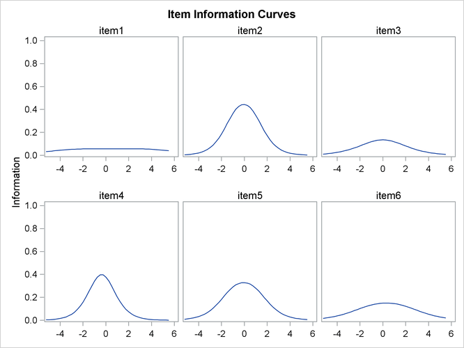
In the context of item response theory, the amount of information that each item or the entire test provides might not be
evenly distributed across the entire continuum of latent constructs. The value of the slope parameter indicates the amount
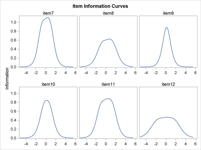
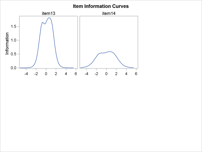
of information that the item provides. For this example, parameter estimates and item information curves are shown in Output 53.4.2 and Output 53.4.3, respectively. By examining the parameter estimates and the item information curves, you can see that items that have high
slope values have tall, narrow information curves. For example, because the slope value of item9 is much larger than the slope value of item1, the information curve is taller and narrower for item9 than it is for item1.
Output 53.4.2: Parameter Estimates
| Item Parameter Estimates | |||||
|---|---|---|---|---|---|
| Response Model |
Item | Parameter | Estimate | Standard Error |
Pr > |t| |
| Graded | item1 | Threshold 1 | -2.09483 | 0.33839 | <.0001 |
| Threshold 2 | 3.20986 | 0.50260 | <.0001 | ||
| Slope | 0.45899 | 0.07087 | <.0001 | ||
| item2 | Threshold 1 | -0.54935 | 0.07526 | <.0001 | |
| Threshold 2 | 0.45190 | 0.07144 | <.0001 | ||
| Slope | 1.22585 | 0.09826 | <.0001 | ||
| item5 | Threshold 1 | -0.71564 | 0.08937 | <.0001 | |
| Threshold 2 | 0.59637 | 0.08419 | <.0001 | ||
| Slope | 1.05329 | 0.08843 | <.0001 | ||
| item6 | Threshold 1 | -0.60606 | 0.11597 | <.0001 | |
| Threshold 2 | 1.18041 | 0.15115 | <.0001 | ||
| Slope | 0.71308 | 0.07648 | <.0001 | ||
| item7 | Threshold 1 | -0.78445 | 0.06313 | <.0001 | |
| Threshold 2 | 0.24069 | 0.05178 | <.0001 | ||
| Threshold 3 | 0.87163 | 0.06538 | <.0001 | ||
| Slope | 1.90616 | 0.12225 | <.0001 | ||
| item8 | Threshold 1 | -0.74471 | 0.07231 | <.0001 | |
| Threshold 2 | 0.60159 | 0.06732 | <.0001 | ||
| Threshold 3 | 1.34996 | 0.09664 | <.0001 | ||
| Slope | 1.43137 | 0.09921 | <.0001 | ||
| item10 | Threshold 1 | -0.33505 | 0.05731 | <.0001 | |
| Threshold 2 | 0.67167 | 0.06498 | <.0001 | ||
| Slope | 1.69974 | 0.12235 | <.0001 | ||
| item11 | Threshold 1 | -1.02908 | 0.07590 | <.0001 | |
| Threshold 2 | -0.03480 | 0.05564 | 0.2659 | ||
| Threshold 3 | 0.64199 | 0.06410 | <.0001 | ||
| Threshold 4 | 1.34486 | 0.08998 | <.0001 | ||
| Slope | 1.67107 | 0.10914 | <.0001 | ||
| item12 | Threshold 1 | -1.87573 | 0.13564 | <.0001 | |
| Threshold 2 | -0.80823 | 0.08484 | <.0001 | ||
| Threshold 3 | -0.09862 | 0.06855 | 0.0751 | ||
| Threshold 4 | 0.59884 | 0.07678 | <.0001 | ||
| Threshold 5 | 1.22786 | 0.10198 | <.0001 | ||
| Threshold 6 | 1.83256 | 0.13657 | <.0001 | ||
| Slope | 1.19488 | 0.08609 | <.0001 | ||
| item13 | Threshold 1 | -0.81329 | 0.05663 | <.0001 | |
| Threshold 2 | 0.31547 | 0.04744 | <.0001 | ||
| Threshold 3 | 1.07939 | 0.06425 | <.0001 | ||
| Slope | 2.49426 | 0.15672 | <.0001 | ||
| item14 | Threshold 1 | -1.37128 | 0.09688 | <.0001 | |
| Threshold 2 | 0.35368 | 0.06259 | <.0001 | ||
| Threshold 3 | 1.35631 | 0.09724 | <.0001 | ||
| Slope | 1.39958 | 0.09563 | <.0001 | ||
| TwoP | item3 | Difficulty | -0.01166 | 0.09635 | 0.4519 |
| Slope | 0.73660 | 0.08604 | <.0001 | ||
| item4 | Difficulty | -0.36507 | 0.06875 | <.0001 | |
| Slope | 1.26289 | 0.11334 | <.0001 | ||
| item9 | Difficulty | 0.16315 | 0.06378 | 0.0053 | |
| Slope | 1.89046 | 0.20555 | <.0001 | ||
For individual items, most of the information concentrates around the area that is defined by the difficulty parameters. The
binary response item provides most of the information around the difficulty parameter. For ordinal items, most of the information
falls in the region between the lowest and the highest threshold parameters. By comparing the information curves for item7 and item9, you can also see that when response items have the same slope value, the ordinal item is more informative than the binary
item.
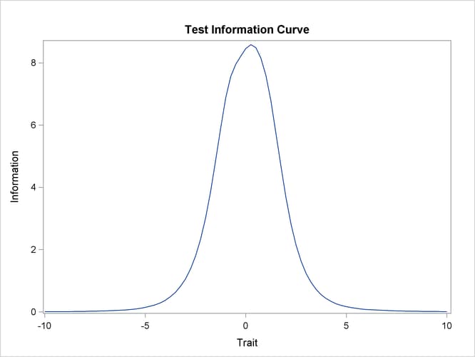
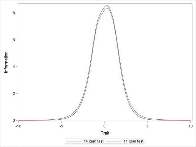
When all items in a test are considered together, the information for measuring the latent trait is called the test information. Test information is computed as a summation of the information that is provided by all the items in the test. Output 53.4.4 includes the test information curve for this example.
Item and test information are very useful for item selection. One important purpose of item selection is to maximize the test information across the continuum of latent construct of interest.
During the item selection process, ideally you want to select highly discriminating items whose threshold parameters cover the range of latent construct of interest. However, in practice you often encounter situations in which these highly discriminating items cannot provide enough information for a specific range of latent construct of interest, especially when these items are binary. In these situations, you might need to select some less discriminating items that can add information to the area that is not covered by these highly discriminating items.
For this example, the slope parameters range from 0.46 to 2.49, and the threshold parameters range from –2.1 to 3.2. Among
these 14 items, three of them (item1, item3, and item6) have slope values less than 1. The slope value for item1 is less than 0.5, which is especially low. The item information curves suggest that these three items provide much less information
than the other items. As a result, you might consider dropping these three items to economize future test administration.
Output 53.4.5 shows the test information curves for the original test, which has 14 items, and the shorter test, which excludes item1, item3, and item6. The two information curves are almost identical, suggesting that the shorter test provides almost the same amount of information
as the longer test. Because the shorter test is more economical, it is preferred for future testing.