Example 53.2 Multidimensional Exploratory and Confirmatory IRT Models
This example illustrates how to use the IRT procedure to fit multidimensional exploratory and confirmatory IRT models. The
data set that is introduced in Example 53.1 is also used here. Two more items, item9 and item10, are added to the data set. These two items are designed to measure subjects’ satisfaction with their friendships and their
family life, respectively.
data IrtMulti;
   input item1-item10 @@;
   datalines;
1 0 0 0 1 1 2 1 2 1 1 1 1 1 1 3 3 3 3 3 0 1 0 0 1 1 1 1 1 1 1 0 0 1 0
1 2 3 2 2 0 0 0 0 0 1 1 1 1 1 1 0 0 1 0 1 3 3 1 2 0 0 0 0 0 1 1 3 3 2
0 0 1 0 0 1 2 2 3 2 0 1 0 0 1 1 1 2 2 2 0 0 0 0 0 2 2 3 3 2 0 1 0 1 0
2 3 3 3 3 0 0 1 0 1 1 2 3 2 3 1 1 1 1 1 2 2 3 2 2 0 0 0 0 1 1 2 2 3 1
1 0 1 1 1 2 3 3 2 3 0 1 0 0 1 1 2 3 3 3 1 0 1 1 1 2 3 3 3 3 0 1 0 1 1
3 2 3 3 2 1 1 1 0 0 1 3 3 2 1 1 1 0 0 1 2 3 3 3 3 0 1 1 1 1 1 2 1 2 3
1 0 0 1 1 3 1 1 1 1 1 0 0 0 1 1 1 3 3 1 0 0 0 0 1 1 3 3 3 3 0 0 0 0 0
1 1 1 3 2 1 0 0 0 0 1 3 3 3 3 1 1 0 1 1 3 1 1 3 3 1 0 1 1 1 1 3 1 1 1

   ... more lines ...

3 3 1 3 2 0 0 0 1 0 1 3 2 2 1 0 0 0 0 1 1 2 2 2 3 1 0 1 0 1 2 2 3 2 1
1 0 0 1 1 1 2 2 3 1 0 1 0 1 0 1 3 1 1 1 0 1 1 0 1 3 3 3 3 2 1 0 1 0 0
1 2 1 1 1 1 0 1 1 0 1 3 3 1 3 1 1 0 1 0 2 2 2 2 3 1 1 0 1 1 3 2 3 2 2
0 0 0 1 0 2 2 3 1 2 0 0 0 1 0 2 3 3 3 2 0 1 0 0 1 2 2 1 2 1
;
Now, suppose that previous research results suggest that two latent factors underlie these 10 items. However, knowledge about
the factor structure is very limited. The first step you can take is to fit an exploratory IRT model by using two factors.
This can be accomplished easily by submitting the following statements:
ods graphics on;
proc irt data=IrtMulti nfactor=2 plots=scree;
   var item1-item10;
run;
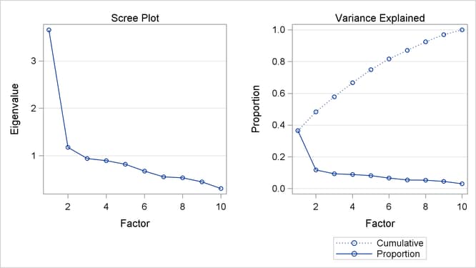
The first table that you want to check is the "Eigenvalue" table, shown in Output 53.2.1. There are only two eigenvalues greater than 1 in this example. This result, to some extent, suggests that two factors might
be enough in this example. Output 53.2.2 include the scree and variance explained plots.
Output 53.2.1: Eigenvalues of the Polychoric Correlation matrix
The IRT Procedure
| 3.65750431 |
2.47883117 |
0.3658 |
0.3658 |
| 1.17867314 |
0.23738137 |
0.1179 |
0.4836 |
| 0.94129177 |
0.04672399 |
0.0941 |
0.5777 |
| 0.89456778 |
0.07508308 |
0.0895 |
0.6672 |
| 0.81948471 |
0.14774320 |
0.0819 |
0.7492 |
| 0.67174151 |
0.12081203 |
0.0672 |
0.8163 |
| 0.55092948 |
0.01698300 |
0.0551 |
0.8714 |
| 0.53394648 |
0.08647230 |
0.0534 |
0.9248 |
| 0.44747418 |
0.14308753 |
0.0447 |
0.9696 |
| 0.30438664 |
|
0.0304 |
1.0000 |
Output 53.2.2: Scree and Variance Explained Plots
If the optimization algorithm converges successfully, the original and rotated slope matrices are produced. The default rotation
method is varimax. You can use the ROTATE=
option in the PROC IRT
statement to specify a different rotation method.
Output 53.2.3: Slope Matrix
| 1.87474 |
0.63566 |
| 1.71878 |
0.56368 |
| 1.29600 |
0.54156 |
| 0.74920 |
0.36351 |
| 0.41017 |
0.63813 |
| 0.44038 |
0.39948 |
| 0.68674 |
1.18496 |
| 0.74058 |
1.97319 |
| 0.40213 |
1.26228 |
| 0.40067 |
1.26536 |
This example uses the default varimax rotation. Output 53.2.3 shows the rotated slope matrices. The rotated slope matrix is displayed in the standard matrix format. From the rotated slope
matrix, you can see that the first factor is mainly reflected by item1 to item4 and item6, and the second factor is mainly reflected by the rest of the items. The exploratory results suggest a hypothesis about the
factor structure of the items. In practice, you might want to confirm this structure by a confirmatory analysis of the new
data. However, for illustration purposes, the same data set is used here to demonstrate the confirmatory model fitting by
using the following statements:
proc irt data=IrtMulti;
   var item1-item4 item6 item5 item7-item10;
   factor  Factor1->item1-item4 item6,
           Factor2->item5 item7-item10;
run;
ods graphics off;
Output 53.2.5 and Output 53.2.4 show the model fit statistics for the confirmatory model and the exploratory model, respectively. Output 53.2.6 shows the slope matrix from this confirmatory analysis. Because the number of response patterns in the data set, 500, is
much lower than the total number of possible response patterns,  , you cannot use Pearson’s chi-square or the likelihood ratio statistic to test the overall fit of the confirmatory model.
If you have two nested models, you can still use the likelihood ratio statistic to test the difference between these two models.
For illustration purposes, assume that the exploratory model and the confirmatory model are two independent models. Because
the confirmatory model is nested within the exploratory model, you can use the likelihood ratio test to compare the two models.
The likelihood ratio test statistic is 132.4. The degree of freedom is 9. The corresponding p-value is 0, which suggests that the difference between these two models is significant. There are many options that you can
use to improve the model fit. For this example, you can try to free some of the fixed slope parameters or free the covariance
between the factors.
Output 53.2.4: Model Fit Statistics for Exploratory Model
The IRT Procedure
| -3993.389529 |
| 8054.7790586 |
| 8198.075734 |
Output 53.2.5: Model Fit Statistics for Confirmatory Model
The IRT Procedure
| -4125.792484 |
| 8301.5849679 |
| 8406.9501703 |
Output 53.2.6: Slope Matrix