The ICLIFETEST Procedure

This example illustrates the use of the ICLIFETEST procedure to estimate the survival function and test for equality of survival functions by using interval-censored data from a breast cancer study.
The data consist of observations on 94 subjects from a retrospective study that compares the risks of breast cosmetic deterioration after tumorectomy (Finkelstein, 1986). There are two treatment groups: patients who receive radiation alone (TRT=RT) and patients who receive radiation plus chemotherapy (TRT=RT+RCT). Patients are followed up every four to six months, leading to interval-censored observations of deterioration times. Of the 94 observation times, 38 are right-censored and the remaining 56 are censored into intervals of finite length.
The following statements create a SAS data set named RT for the group that receives radiation alone. The variable lTime provides the last follow-up time at which cosmetic deterioration has not occurred for the patient, and the variable rTime provides the last follow-up time immediately after the event. Note that for the ICLIFETEST procedure to recognize the observations
as right-censored, their right bounds must be represented by missing values in the input data set.
data RT;
   input lTime rTime @@;
   trt = 'RT    ';
   datalines;
45  .  25 37  37  .
 6 10  46  .   0  5
 0  7  26 40  18  .
46  .  46  .  24  .
46  .  27 34  36  .
 7 16  36 44   5 11
17  .  46  .  19 35
 7 14  36 48  17 25
37 44  37  .  24  .
 0  8  40  .  32  .
 4 11  17 25  33  .
15  .  46  .  19 26
11 15  11 18  37  .
22  .  38  .  34  .
46  .   5 12  36  .
46  .
;
The following statements create a SAS data set named RCT for patients who receive both radiation and chemotherapy:
data RCT;
   input lTime rTime @@;
   trt = 'RT+RCT';
   datalines;
 8 12   0  5  30 34
 0 22   5  8  13  .
24 31  12 20  10 17
17 27  11  .   8 21
17 23  33 40   4  9
24 30  31  .  11  .
16 24  13 39  14 19
13  .  19 32   4  8
11 13  34  .  34  .
16 20  13  .  30 36
18 25  16 24  18 24
17 26  35  .  16 60
32  .  15 22  35 39
23  .  11 17  21  .
44 48  22 32  11 20
14 17  10 35  48  .
;
The following statements combine the data sets RT and RCT into a single data set named BCS that is to be analyzed by the ICLIFETEST procedure:
data BCS;
   set RT RCT;
run;
Suppose you want to gain insights into the incidence rate of cosmetic deterioration over time after the two treatments. From the perspective of survival analysis, the tasks are to estimate the survival probabilities for the two treatment groups and to test for a systematic difference between the groups.
The following statements invoke the ICLIFETEST procedure to estimate the survival functions for both treatment groups:
ods graphics on;
proc iclifetest plots=(survival logsurv) data=BCS impute(seed=1234);
   strata trt;
   time (lTime, rTime);
run;
In the TIME statement, the variables that represent the interval boundaries, lTime and rTime, are enclosed in parentheses and separated by a comma. Because the treatment indicator variable, Trt, is specified in the STRATA statement, PROC ICLIFETEST conducts the analysis separately for each treatment group. When you
specify the keywords SURVIVAL and LOGSURV in the PLOTS= option, the procedure plots the estimated survival functions and the
negative of the log transformations of the estimates. You can specify an integer seed for the random number generator that
is used in creating imputed data sets for calculating standard errors of the survival estimates. If the SEED= option is not
specified, a random seed is obtained from the computer’s clock. For more information about the IMPUTE option, see the section
IMPUTE <phrase remap="Optional">(<phrase remap="Argument">options</phrase>)</phrase>.
Figure 50.1 displays the nonparametric survival estimates for the radiation group (TRT=RT).
Figure 50.1: Nonparametric Survival Estimates
| Nonparametric Survival Estimates | ||||
|---|---|---|---|---|
| Probability Estimate | Imputation Standard Error |
|||
| Time Interval | Failure | Survival | ||
| 0 | 4 | 0.0000 | 1.0000 | 0.0000 |
| 5 | 6 | 0.0463 | 0.9537 | 0.0354 |
| 7 | 7 | 0.0797 | 0.9203 | 0.0458 |
| 8 | 11 | 0.1684 | 0.8316 | 0.0580 |
| 12 | 24 | 0.2391 | 0.7609 | 0.0629 |
| 25 | 33 | 0.3318 | 0.6682 | 0.0706 |
| 34 | 38 | 0.4136 | 0.5864 | 0.0739 |
| 40 | 46 | 0.5344 | 0.4656 | 0.0758 |
| 48 | Inf | 1.0000 | 0.0000 | 0.0000 |
Note that because interval censoring is present, the nonparametric estimates of failure probability and survival probability
are computed for a set of nonoverlapping intervals. These estimates are constant within each interval. For example, consider
the time interval ![]() . The estimated failure probability is 0.1684 between 8 and 11. The interval
. The estimated failure probability is 0.1684 between 8 and 11. The interval ![]() , which is not displayed, is an interval for which the survival estimate cannot be uniquely determined; such intervals are
referred to as Turnbull intervals. The failure probability increases to 0.2391 at 12 and remains constant until 24. The table
in Figure 50.1 also contains standard errors for the estimates. For a plot of the survival probabilities, see Figure 50.4.
, which is not displayed, is an interval for which the survival estimate cannot be uniquely determined; such intervals are
referred to as Turnbull intervals. The failure probability increases to 0.2391 at 12 and remains constant until 24. The table
in Figure 50.1 also contains standard errors for the estimates. For a plot of the survival probabilities, see Figure 50.4.
Figure 50.2 displays estimated quartiles of the deterioration time and corresponding 95% confidence limits for the group that receives radiation only.
Because the estimated failure distribution is undefined inside the Turnbull intervals, the quartiles of deterioration time and their confidence intervals are obtained by imputing probabilities within the intervals. This approach is ad hoc in nature, so the results should be interpreted with caution. For more information, see the section Quartile Estimation.
The ICLIFETEST procedure also produces a summary of the frequencies of various types of censoring (Figure 50.3).
The categories are exact times, left-censoring, right-censoring, and interval-censoring. The percentage of each category within a stratum is also calculated.
Figure 50.4 displays the estimated survival functions for the two treatments.
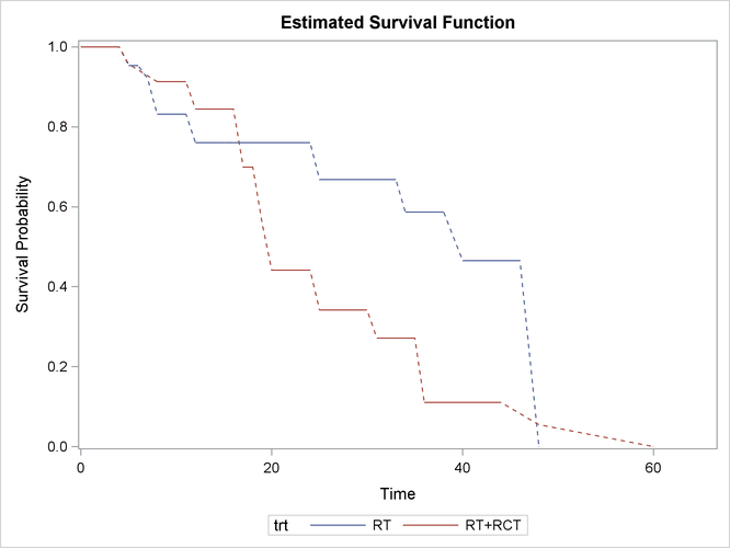
Clearly, the group that receives radiation alone tends to survive longer before experiencing cosmetic deterioration than the group that receives both radiation and chemotherapy. As shown in Figure 50.1, the estimated survival probabilities are undetermined within the Turnbull intervals. For ease of visualization, dashed lines are plotted across the Turnbull intervals for which the estimates are not defined. You can suppress plotting of the dashed lines by specifying the NODASH option. For more information about options for customizing the survival plots, see the section SURVIVAL <phrase remap="Optional">(CL | FAILURE | NODASH | STRATA | TEST)</phrase>.
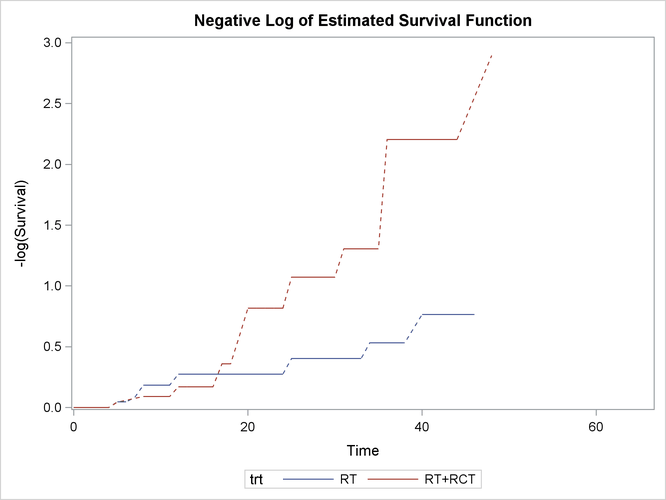
Figure 50.5 displays log transformations of the survival estimates over time.
The following statements formally test whether patients in the two treatment groups have the same survival rate. By default, the generalized log-rank test with constant weights over time is used. For more information about alternative weight functions, see the section Generalized Log-Rank Statistic. You can specify an integer seed for the random number generator that is used in creating imputed data sets for obtaining standard errors of the survival estimates and for calculating the generalized log-rank test. If the SEED= option is not specified, a random seed is obtained from the computer’s clock.
proc iclifetest data=BCS impute(seed=1234);
   time (lTime, rTime);
   test trt;
run;
Figure 50.6 displays results of the generalized log-rank test.
The chi-square statistic for the generalized log-rank test is 7.3349. The p-value of 0.0068 is computed using the chi-square distribution with one degree of freedom.