Statistical Methods :: SAS/STAT(R) 13.2 User's Guide

Nonparametric Estimation of the Survival Function

Suppose the event times for a total of n subjects, $T_1$ , $T_2$ , …, $T_ n$ , are independent random variables with an underlying cumulative distribution function $F(t)$ . Denote the corresponding survival function as $S(t)$ . Interval-censoring occurs when some or all $T_ i$ ’s cannot be observed directly but are known to be within the interval $(L_ i, R_ i], L_ i \le R_ i$ .

The observed intervals might or might not overlap. It they do not overlap, then you can usually use conventional methods for right-censored data, with minor modifications. On the other hand, if some intervals overlap, you need special algorithms to compute an unbiased estimate of the underlying survival function.

To characterize the nonparametric estimate of the survival function, Peto (1973) and Turnbull (1976) show that the estimate can jump only at the right endpoint of a set of nonoverlapping intervals (also known as Turnbull intervals), $\{ I_ j=(q_ j, p_ j], j=1,\ldots ,m \}$ . A simple algorithm for finding these intervals is to order all the boundary values $\{ L_ i,R_ i, i=1,\ldots ,n\}$ with labels of L and R attached and then pick up the intervals that have L as the left boundary and R as the right boundary. For example, suppose that the data set contains only three intervals, $(1,3]$ , $(2,4]$ , and $(5,6]$ . The ordered values are $1(L), 2(L), 3(R), 4(R), 5(L), 6(R)$ . Then the Turnbull intervals are $(2,3]$ and $(5,6]$ .

For the exact observation $L_ i=R_ i=t$ , Ng (2002) suggests that it be represented by the interval $(t-\epsilon , t)$ for a positive small value $\epsilon$ . If $R_ j=t$ for an observation $(L_ j, R_ j]$ ( $L_ j<R_ j$ ), then the observation is represented by $(L_ j+\epsilon , R_ j-\epsilon )$ .

Define $\theta _ j = P(T \in I_ j)$ , $j=1,\ldots ,m$ . Given the data, the survival function, $S(t)$ , can be determined only up to equivalence classes t, which are complements of the Turnbull intervals. $S(t)$ is undefined if t is within some $I_ j$ . The likelihood function for $\btheta = \{ \theta _ j, j=1,\ldots ,m \}$ is then

$L(\btheta ) = \prod _{i=1}^{n} \Big( \sum _{j=1}^{m} \alpha _{ij} \theta _ j \Big)$

where $\alpha _{ij}$ is 1 if $I_ j$ is contained in $(L_ i, R_ i]$ and 0 otherwise.

Denote the maximum likelihood estimate for $\hat{\btheta }$ as $\hat{\btheta } = \{ \hat{\theta }_ j, j=1,\ldots ,m\}$ . The survival function can then be estimated as

$\hat{S}(t) = \sum _{k: p_ k>t} \hat{\theta }_ k, \ \ \ t \not\in \mr{any} \ I_ j, j=1,\ldots ,m$

Estimation Algorithms

Peto (1973) suggests maximizing this likelihood function by using a Newton-Raphson algorithm subject to the constraint $\sum _{i=j}^{m} \theta _ j = 1$ . This approach has been implemented in the $\%$ ICE macro. Although feasible, the optimization becomes less stable as the dimension of $\btheta$ increases.

Treating interval-censored data as missing data, Turnbull (1976) derives a self-consistent equation for estimating the $\theta _ j$ ’s:

$\theta _ j = \frac{1}{n} \sum _{i=1}^{n} \mu _{ij}(\btheta ) = \frac{1}{n} \sum _{i=1}^{n} \frac{\alpha _{ij}\theta _ j}{\sum _{j=1}^{m} \alpha _{ij}\theta _ j}$

where $\mu _{ij}(\btheta )$ is the expected probability that the event $T_ i$ occurs within $I_ j$ for the ith subject, given the observed data.

The algorithm is an expectation-maximization (EM) algorithm in the sense that it iteratively updates $\btheta$ and $\mu _{ij}(\btheta )$ . Convergence is declared if, for a chosen number $\epsilon >0$ ,

$\sum _{j=1}^{m} | \hat{\theta }_ j^{(l)} - \hat{\theta }_ j^{(l-1)} | < \epsilon$

where $\hat{\theta }_ j^{(l)}$ denotes the updated value for $\theta _ j$ after the lth iteration.

An alternative criterion is to declare convergence when increments of the likelihood are small:

$| L(\hat{\theta }_ j^{(l)}; j=1,\ldots ,m) - L(\hat{\theta }_ j^{(l-1)}; j=1,\ldots ,m) | < \epsilon$

There is no guarantee that the converged values constitute a maximum likelihood estimate (MLE). Gentleman and Geyer (1994) introduced the Kuhn-Tucker conditions based on constrained programming as a check of whether the algorithm converges to a legitimate MLE. These conditions state that a sufficient and necessary condition for the estimate to be a MLE is that the Lagrange multipliers $\gamma _ j = n-c_ j$ are nonnegative for all the $\theta _ j$ ’s that are estimated to be zero, where $c_ j$ is the derivative of the log-likelihood function with respect to $\theta _ j$ :

$c_ j = \frac{\partial \log (L)}{\partial \theta _ j} = \sum _{i=1}^{n} \frac{\alpha _{ij}}{\sum _{j=1}^{m} \alpha _{ij}\theta _ j}$

You can use Turnbull’s method by specifying METHOD=TURNBULL in the ICLIFETEST statement. The Lagrange multipliers are displayed in the "Nonparametric Survival Estimates" table.

Groeneboom and Wellner (1992) propose using the iterative convex minorant (ICM) algorithm to estimate the underlying survival function as an alternative to Turnbull’s method. Define $\beta _ j = F(p_ j)$ , $j=1,\ldots ,m$ as the cumulative probability at the right boundary of the jth Turnbull interval: $\beta _ j = \sum _{k=1}^{j} \theta _ k$ . It follows that $\beta _ m = 1$ . Denote $\beta _0 = 0$ and $\bbeta = (\beta _1,\ldots ,\beta _{m-1})’$ . You can rewrite the likelihood function as

$L(\bbeta ) = \prod _{i=1}^{n} \sum _{j=1}^{m} \alpha _{ij}(\beta _ j - \beta _{j-1})$

Maximizing the likelihood with respect to the $\theta _ j$ ’s is equivalent to maximizing it with respect to the $\beta _ j$ ’s. Because the $\beta _ j$ ’s are naturally ordered, the optimization is subject to the following constraint:

$C = \{ \mb{x}=(\beta _1,\ldots ,\beta _{m-1}): 0 \le \beta _1 \le \cdots \le \beta _{m-1} \le 1 \}$

Denote the log-likelihood function as $l(\bbeta )$ . Suppose its maximum occurs at $\hat{\bbeta }$ . Mathematically, it can be proved that $\hat{\bbeta }$ equals the maximizer of the following quadratic function:

$g^*(\mb{x}|\mb{y},\mb{W}) = -\frac{1}{2} (\mb{x}-\mb{y})’ \mb{W} (\mb{x}-\mb{y})$

where $\mb{y}=\hat{\bbeta }+\mb{W}^{-1} \nabla l(\hat{\bbeta })$ , $\nabla l(\cdot )$ denotes the derivatives of $l(\cdot )$ with respect to $\bbeta$ , and $\mb{W}$ is a positive definite matrix of size $(m-1)\times (m-1)$ (Groeneboom and Wellner, 1992).

An iterative algorithm is needed to determine $\hat{\bbeta }$ . For the lth iteration, the algorithm updates the quantity

$\mb{y}^{(l)}=\hat{\bbeta }^{(l-1)} - \mb{W}^{-1}(\hat{\bbeta }^{(l-1)}) \nabla l(\hat{\bbeta }^{(l-1)})$

where $\hat{\bbeta }^{(l-1)}$ is the parameter estimate from the previous iteration and $\mb{W}(\hat{\bbeta }^{(l-1)})=\mr{diag}(w_ j,j=1,\ldots ,m-1)$ is a positive definite diagonal matrix that depends on $\hat{\bbeta }^{(l-1)}$ .

A convenient choice for $\mb{W}(\bbeta )$ is the negative of the second-order derivative of the log-likelihood function $l(\bbeta )$ :

$w_ j = w_ j(\bbeta ) = - \frac{\partial ^2}{\partial \beta _ j^2} l(\bbeta )$

Given $\mb{y}=\mb{y}^{(l)}=(y_1^{(l)},\ldots ,y_{m-1}^{(l)})’$ and $\mb{W}=\mb{W}(\hat{\bbeta }^{(l-1)})$ , the parameter estimate for the lth iteration $\hat{\bbeta }^{(l)}$ maximizes the quadratic function $g^*(\mb{x}|\mb{y},\mb{W})$ .

Define the cumulative sum diagram $\{ P_ k,k=0,\ldots ,m-1\}$ as a set of m points in the plane, where $P_0=(0,0)$ and

$P_ k = \Big( \sum _{i=1}^{k} w_ i, \sum _{i=1}^{k} w_ i y_ i^{(l)} \Big)$

Technically, $\hat{\bbeta }^{(l)}$ equals the left derivative of the convex minorant, or in other words, the largest convex function below the diagram $\{ P_ k,k=0,\ldots ,m-1\}$ . This optimization problem can be solved by the pool-adjacent-violators algorithm (Groeneboom and Wellner, 1992).

Occasionally, the ICM step might not increase the likelihood. Jongbloed (1998) suggests conducting a line search to ensure that positive increments are always achieved. Alternatively, you can switch to the EM step, exploiting the fact that the EM iteration never decreases the likelihood, and then resume iterations of the ICM algorithm after the EM step. As with Turnbull’s method, convergence can be determined based on the closeness of two consecutive sets of parameter values or likelihood values. You can use the ICM algorithm by specifying METHOD=ICM in the PROC ICLIFETEST statement.

As its name suggests, the EMICM algorithm combines the self-consistent EM algorithm and the ICM algorithm by alternating the two different steps in its iterations. Wellner and Zhan (1997) show that the converged values of the EMICM algorithm always constitute an MLE if it exists and is unique. The ICLIFETEST procedure uses the EMICM algorithm as the default.

Variance Estimation of the Survival Estimator

Peto (1973) and Turnbull (1976) suggest estimating the variances of the survival estimates by inverting the Hessian matrix, which is obtained by twice differentiating the log-likelihood function. This method can become less stable when the number of $\theta _ j$ ’s increase as n increases. Simulations have shown that the confidence limits based on variances estimated with this method tend to have conservative coverage probabilities that are greater than the nominal level (Goodall, Dunn, and Babiker, 2004).

Sun (2001) proposes using two resampling techniques, simple bootstrap and multiple imputation, to estimate the variance of the survival estimator. The undefined regions that the Turnbull intervals represent create a special challenge using the bootstrap method. Because each bootstrap sample could have a different set of Turnbull intervals, some time points to evaluate the variances based on the original Turnbull intervals might be located within the intervals in a bootstrap sample, with the result that their survival probabilities become unknown. A simple ad hoc solution is to shrink the Turnbull interval to its right boundary and modify the survival estimates into a right continuous function:

$\hat{S}_ m(t) = \sum _{j:p_ j>t} \hat{\theta }_ j$

Let M denote the number of resampling data sets. Let $A_1^ k,\ldots ,A_ n^ k$ denote the n independent samples from the original data with replacement, $k=1,\ldots ,M$ . Let $\hat{S}_ m^ k(t)$ be the modified estimate of the survival function computed from the kth resampling data set. Then you can estimate the variance of $\hat{S}(t)$ by the sample variance as

$\hat{\sigma }^2_{b} (t) = \frac{1}{M-1} \sum _{k=1}^{M} [ \hat{S}_ m^ k(t) - \bar{S}_ m(t) ]^2$

where

$\bar{S}_ m (t) = \frac{\sum _{k=1}^{M} \hat{S}_ m^ k(t)}{M}$

The method of multiple imputations exploits the fact that interval-censored data reduce to right-censored data when all interval observations of finite length shrink to single points. Suppose that each finite interval has been converted to one of the $p_ j$ values it contains. For this right-censored data set, you can estimate the variance of the survival estimates via the well-known Greenwood formula (1958) as

$\hat{\sigma }_ G^2 (t) = \hat{S}_{KM}^2(t) \sum _{q_ j < t} \frac{d_ j}{n_ j (n_ j - d_ j)}$

where $d_ j$ is the number of events at time $p_ j$ and $n_ j$ is the number of subjects at risk just prior to $p_ j$ , and $\hat{S}_{KM}(t)$ is the Kaplan-Meier estimator of the survival function,

$\hat{S}_{KM} (t) = \prod _{q_ j<t} \frac{n_ j - d_ j}{n_ j}$

Essentially, multiple imputation is used to account for the uncertainty of ranking overlapping intervals. The kth imputed data set is obtained by substituting every interval-censored observation of finite length with an exact event time randomly drawn from the conditional survival function:

$\hat{S}_ i(t) = \frac{\hat{S}_ m(t) - \hat{S}_ m(R_ i+)}{\hat{S}_ m(L_ i) - \hat{S}_ m(R_ i+)}, \ \ \ t \in (L_ i, R_ i]$

Because $\hat{S}_ m(t)$ only jumps at the $p_ j$ , this is a discrete function.

Denote the Kaplan-Meier estimate of each imputed data set as $\hat{S}_{KM}^ k(t)$ . The variance of $\hat{S}(t)$ is estimated by

$\hat{\sigma }^2_{I}(t) = \hat{S}^2(t) \sum _{q_ j < t} \frac{d_ j'}{n_ j'(n_ j' - d_ j')} + \frac{1}{M-1} \sum _{k=1}^{M} [\hat{S}_{KM}^ k(t) - \bar{S}_{KM}(t)]$

where

$\bar{S}_{KM}(t) = \frac{1}{M} \sum _{k=1}^{M} \hat{S}_{KM}^ k (t)$

and

$d_ j’ = \sum _{i=1}^{n} \frac{\alpha _{ij} [\hat{S}(p_{j-1}) - \hat{S}(p_ j)]}{\sum _{j=1}^{m} \alpha _{ij} [\hat{S}(p_{j-1}) - \hat{S}(p_ j)]}$

and

$n_ j’ = \sum _{k=j}^{m} d_ j’$

Note that the first term in the formula for $\hat{\sigma }^2_{I}(t)$ mimics the Greenwood formula but uses expected numbers of deaths and subjects. The second term is the sample variance of the Kaplan-Meier estimates of imputed data sets, which accounts for between-imputation contributions.

Pointwise Confidence Limits of the Survival Function

Pointwise confidence limits can be computed for the survival function given the estimated standard errors. Let $\alpha$ be specified by the ALPHA= option. Let $z_{\alpha / 2}$ be the critical value for the standard normal distribution. That is, $\Phi (-z_{\alpha / 2}) = \alpha / 2$ , where $\Phi$ is the cumulative distribution function of the standard normal random variable.

Constructing the confidence limits for the survival function $S(t)$ as $\hat{S}(t) \pm z_{\alpha / 2}\hat{\sigma }[\hat{S}(t)]$ might result in an estimate that exceeds the range [0,1] at extreme values of t. This problem can be avoided by applying a transformation to $S(t)$ so that the range is unrestricted. In addition, certain transformed confidence intervals for $S(t)$ perform better than the usual linear confidence intervals (Borgan and Liestøl, 1990). You can use the CONFTYPE= option to set one of the following transformations: the log-log function (Kalbfleisch and Prentice, 1980), the arcsine–square root function (Nair, 1984), the logit function (Meeker and Escobar, 1998), the log function, and the linear function.

Let g denote the transformation that is being applied to the survival function $S(t)$ . Using the delta method, you estimate the standard error of $g(\hat{S}(t))$ by

$\tau (t) = \hat{\sigma }\left[g(\hat{S}(t))\right] = g’\left(\hat{S}(t)\right)\hat{\sigma }[\hat{S}(t)]$

where g’ is the first derivative of the function g. The 100(1 – $\alpha$ )% confidence interval for $S(t)$ is given by

$g^{-1}\left\{ g[\hat{S}(t)] \pm z_{\frac{\alpha }{2}} g’[\hat{S}(t)]\hat{\sigma }[\hat{S}(t)] \right\}$

where $g^{-1}$ is the inverse function of g. The choices for the transformation g are as follows:

arcsine–square root transformation: The estimated variance of $\sin ^{-1}\left(\sqrt {\hat{S}(t)}\right)$ is $\hat{\tau }^2(t) = \frac{\hat{\sigma }^2[\hat{S}(t)]}{4\hat{S}(t)[1- \hat{S}(t)] }.$ The 100(1 – $\alpha$ )% confidence interval for $S(t)$ is given by

$\sin ^2\left\{ \max \left[0,\sin ^{-1}(\sqrt {\hat{S}(t)}) - z_{\frac{\alpha }{2}} \hat{\tau }(t)\right]\right\} \le S(t) \le \sin ^2\left\{ \min \left[\frac{\pi }{2},\sin ^{-1}(\sqrt {\hat{S}(t)}) + z_{\frac{\alpha }{2}} \hat{\tau }(t)\right]\right\}$
linear transformation: This is the same as the identity transformation. The 100(1 – $\alpha$ )% confidence interval for $S(t)$ is given by

$\hat{S}(t) - z_{\frac{\alpha }{2}}\hat{\sigma }\left[\hat{S}(t)\right] \le S(t) \le \hat{S}(t) + z_{\frac{\alpha }{2}}\hat{\sigma }\left[\hat{S}(t)\right]$
log transformation: The estimated variance of $\log (\hat{S}(t))$ is $\hat{\tau }^2(t) = \frac{\hat{\sigma }^2(\hat{S}(t))}{\hat{S}^2(t)}.$ The 100(1 – $\alpha$ )% confidence interval for $S(t)$ is given by

$\hat{S}(t)\exp \left(-z_{\frac{\alpha }{2}}\hat{\tau }(t)\right) \le S(t) \le \hat{S}(t)\exp \left(z_{\frac{\alpha }{2}}\hat{\tau }(t)\right)$
log-log transformation: The estimated variance of $\log (-\log (\hat{S}(t))$ is $\hat{\tau }^2(t) = \frac{\hat{\sigma }^2[\hat{S}(t)]}{ [\hat{S}(t)\log (\hat{S}(t))]^2 }.$ The 100(1 – $\alpha$ )% confidence interval for $S(t)$ is given by

$\left[\hat{S}(t)\right]^{\exp \left( z_{\frac{\alpha }{2}} \hat{\tau }(t)\right)} \le S(t) \le \left[\hat{S}(t)\right]^{\exp \left(-z_{\frac{\alpha }{2}} \hat{\tau }(t)\right)}$
logit transformation: The estimated variance of $\log \left(\frac{\hat{S}(t)}{1-\hat{S}(t)}\right)$ is

$\hat{\tau }^2(t) = \frac{\hat{\sigma }^2(\hat{S}(t))}{\hat{S}^2(t)[1- \hat{S}(t)]^2}$

The 100(1 – $\alpha$ )% confidence limits for $S(t)$ are given by

$\frac{\hat{S}(t)}{\hat{S}(t) + \left[1 -\hat{S}(t) \right] \exp \left(z_{\frac{\alpha }{2}}\hat{\tau }(t)\right)} \le S(t) \le \frac{\hat{S}(t)}{\hat{S}(t) + \left[1 -\hat{S}(t) \right] \exp \left(-z_{\frac{\alpha }{2}}\hat{\tau }(t)\right)}$

Quartile Estimation

The first quartile (25th percentile) of the survival time is the time beyond which 75% of the subjects in the population under study are expected to survive. For interval-censored data, it is problematic to define point estimators of the quartiles based on the survival estimate $\hat{S}(t)$ because of its undefined regions of Turnbull intervals. To overcome this problem, you need to impute survival probabilities within the Turnbull intervals. The previously defined estimator $\hat{S}_ m(t)$ achieves this by placing all the estimated probabilities at the right boundary of the interval. The first quartile is estimated by

$q_{.25} = \mr{min}\{ t_ j | \hat{S}_ m(t_ j) < 0.75\}$

If $\hat{S}_ m(t)$ is exactly equal to 0.75 from $t_ j$ to $t_{j+1}$ , the first quartile is taken to be $(t_ j + t_{j+1})/2$ . If $\hat{S}_ m(t)$ is greater than 0.75 for all values of t, the first quartile cannot be estimated and is represented by a missing value in the printed output.

The general formula for estimating the 100p percentile point is

$q_{p} = \mr{min}\{ t_ j | \hat{S}_ m(t_ j) < 1-p\}$

The second quartile (the median) and the third quartile of survival times correspond to p = 0.5 and p = 0.75, respectively.

Brookmeyer and Crowley (1982) constructed the confidence interval for the median survival time based on the confidence interval for the survival function $S(t)$ . The methodology is generalized to construct the confidence interval for the 100p percentile based on a g-transformed confidence interval for $S(t)$ (Klein and Moeschberger, 1997). You can use the CONFTYPE= option to specify the g-transformation. The $100(1-\alpha )$ % confidence interval for the first quantile survival time is the set of all points t that satisfy

$\biggl | \frac{ g(\hat{S}_ m(t)) - g(1 - 0.25)}{g'(\hat{S}_ m(t)) \hat{\sigma }(\hat{S}(t))} \biggr | \leq z_{1-\frac{\alpha }{2}}$

where $g’(x)$ is the first derivative of $g(x)$ and $z_{1-\frac{\alpha }{2}}$ is the $100(1-\frac{\alpha }{2})$ percentile of the standard normal distribution.

Kernel-Smoothed Estimation

After you obtain the survival estimate $\hat{S}(t)$ , you can construct a discrete estimator for the cumulative hazard function. First, you compute the jumps of the discrete function as

$\hat{\lambda }_ j = \frac{c_ j \hat{\theta }_ j }{\sum _{k=j}^{m} c_ k \hat{\theta }_ k}, \ \ j=1,\ldots ,m$

where the $c_ j$ ’s have been defined previously for calculating the Lagrange multiplier statistic.

Essentially, the numerator and denominator estimate the number of failures and the number at risks that are associated with the Turnbull intervals. Thus these quantities estimate the increments of the cumulative hazard function over the Turnbull intervals.

The estimator of the cumulative hazard function is

$\hat{\lambda }(t) = \sum _{k: p_ k<t} \hat{\lambda }_ k, \ \ \ t \not\in \mr{any} \ I_ j$

Like $\hat{S}(t)$ , $\hat{\lambda }(t)$ is undefined if t is located within some Turnbull interval $I_ j$ . To facilitate applying the kernel-smoothed methods, you need to reformulate the estimator so that it has only point masses. An ad hoc approach would be to place all the mass for a Turnbull interval at the right boundary. The kernel-based estimate of the hazard function is computed as

$\tilde{h} (t, b) = -\frac{1}{b} \sum _{j=1}^{m} K \Big( \frac{t-p_ j}{b} \Big) \hat{\lambda }_ j$

where $K(\cdot )$ is a kernel function and $b>0$ is the bandwidth. You can estimate the cumulative hazard function by integrating $\tilde{h} (t, b)$ with respect to t.

Practically, an upper limit $t_ D$ is usually imposed so that the kernel-smoothed estimate is defined on $(0, t_ D)$ . The ICLIFETEST procedure sets the value depending on whether the right boundary of the last Turnbull interval is finite or not: $t_ D=p_ m$ if $p_ m < \infty$ and $t_ D=1.2*q_ m$ otherwise.

Typical choices of kernel function are as follows:

uniform kernel:

$K_ U(x) = \frac{1}{2}, ~ ~ -1\leq x \leq 1\\$
Epanechnikov kernel:

$K_ E(x) = \frac{3}{4}(1-x^2), ~ ~ -1\leq x \leq 1$
biweight kernel:

$K_{\mi{BW}}(x) = \frac{15}{16}(1-x^2)^2, ~ ~ -1\leq x \leq 1$

For t < b, the symmetric kernels $K()$ are replaced by the corresponding asymmetric kernels of Gasser and Müller (1979). Let $q=\frac{t}{b}$ . The modified kernels are as follows:

uniform kernel:

$K_{U,q}(x) = \frac{4(1+q^3)}{(1+q)^4} + \frac{6(1-q)}{(1+q)^3}x, ~ ~ ~ -1 \leq x \leq q$
Epanechnikov kernel:

$K_{E,q}(x)= K_ E(x) \frac{64(2-4q+6q^2-3q^3) + 240(1-q)^2 x }{ (1+q)^4(19-18q+3q^2)}, ~ ~ -1 \leq x \leq q$
biweight kernel:

$K_{\mi{BW},q}(x) = K_{\mi{BW}}(x) \frac{64(8-24q+48q^2-45q^3+15q^4) + 1120(1-q)^3 x}{(1+q)^5(81-168q+126q^2-40q^3+5q^4)}, ~ ~ -1\leq x \leq q$

For $t_ D -b \leq t \leq t_ D$ , let $q=\frac{t_ D - t}{b}$ . The asymmetric kernels for $t<b$ are used, with x replaced by –x.

The bandwidth parameter b controls how much “smoothness” you want to have in the kernel-smoothed estimate. For right-censored data, a commonly accepted method of choosing an optimal bandwidth is to use the mean integrated square error(MISE) as an objective criteria. This measure becomes difficult to adapt to interval-censored data because it no longer has a closed-form mathematical formula.

Pan (2000) proposes using a V-fold cross validation likelihood as a criterion for choosing the optimal bandwidth for the kernel-smoothed estimate of the survival function. The ICLIFETEST procedure implements this approach for smoothing the hazard function. Computing such a criterion entails a cross validation type procedure. First, the original data $\mc{D}$ are partitioned into V almost balanced subsets $\mc{D}^{(v)}$ , $v=1,\ldots ,V$ . Denote the kernel-smoothed estimate of the leave-one-subset-out data $\mc{D}-\mc{D}^{(v)}$ as $\hat{h}^{*(-v)}(t;b)$ . The optimal bandwidth is defined as the one that maximizes the cross validation likelihood:

$b_0 = \mbox{argmax}_{\substack{b}} \sum _{v=1}^{V} L(\hat{h}^{*(-v)}(t;b) | \mc{D}^{(v)})$

Comparison of Survival between Groups

If the TEST statement is specified, the ICLIFETEST procedure compares the K groups formed by the levels of the TEST variable using a generalized log-rank test. Let $S_ k(t)$ be the underlying survival function of the kth group, $k=1,\ldots ,K$ . The null and alternative hypotheses to be tested are

$H_0\colon S_1(t)= S_2(t) = \cdots = S_ K(t)$ for all t

versus

$H_1\colon$ at least one of the $S_ k(t)$ ’s is different for some t

Let $N_ k$ denote the number of subjects in group k, and let n denote the total number of subjects ( $n=N_1+\cdots +N_ K$ ).

Generalized Log-Rank Statistic

For the ith subject, let $\mb{z}_ i=(z_{i1},\ldots ,z_{iK})’$ be a vector of K indicators that represent whether or not the subject belongs to the kth group. Denote $\bbeta =(\beta _1,\ldots ,\beta _ K)’$ , where $\beta _ k$ represents the treatment effect for the kth group. Suppose that a model is specified and the survival function for the ith subject can be written as

$S(t|\mb{z}_ i) = S(t|\mb{z}_ i’\bbeta , \bgamma )$

where $\bgamma$ denotes the nuisance parameters.

It follows that the likelihood function is

$L = \prod _{i=1}^{n} [S(L_ i|\mb{z}_ i’\bbeta , \bgamma ) - S(R_ i|\mb{z}_ i’\bbeta , \bgamma )]$

where $(L_ i, R_ i)$ denotes the interval observation for the ith subject.

Testing whether or not the survival functions are equal across the K groups is equivalent to testing whether all the $\beta _ j$ ’s are zero. It is natural to consider a score test based on the specified model (Finkelstein, 1986).

The score statistics for $\bbeta$ are derived as the first-order derivatives of the log-likelihood function evaluated at $\bbeta =\mb{0}$ and $\hat{\bgamma }$ .

$\mb{U} = (U_1,\ldots ,U_ K)’ = \frac{\partial \log (L)}{\partial \bbeta } \Big|_{\bbeta =\mb{0}, \hat{\bgamma }}$

where $\hat{\bgamma }$ denotes the maximum likelihood estimate for the $\bgamma$ , given that $\bbeta =\mb{0}$ .

Under the null hypothesis that $\bbeta =\mb{0}$ , all K groups share the same survival function $S(t)$ . It is typical to leave $S(t)$ unspecified and obtain a nonparametric maximum likelihood estimate $\hat{S}(t)$ using, for instance, Turnbull’s method. In this case, $\bgamma$ represents all the parameters to be estimated in order to determine $\hat{S}(t)$ .

Suppose the given data generates m Turnbull intervals as $\{ I_ j=(q_ j,p_ j], j=1,\ldots ,m\}$ . Denote the probability estimate at the right end point of the jth interval by $\hat{\theta }_ j$ . The nonparametric survival estimate is $\hat{S}(t)=\sum _{k:p_ k>t} \hat{\theta }_ k$ for $t \not\in$ any $I_ j$ .

Under the null hypothesis, Fay (1999) showed that the score statistics can be written in the form of a weighted log-rank test as

$U_ k = \sum _{j=1}^{m} U_{kj} = \sum _{j=1}^{m} v_ j \left( d_{kj}’ - \frac{n_{kj}'}{n_ j'} d_ j’ \right)$

where

$v_ j = \frac{[\hat{S}(p_ j)-\hat{S}'(p_{j-1})] [\hat{S}(p_{j-1})-\hat{S}'(p_{j})]}{\hat{S}(p_ j)[\hat{S}(p_{j-1})-\hat{S}(p_{j})]}$

and $S’(t)$ denotes the derivative of $S(t)$ with respect to $\bbeta$ .

$d_{kj}’$ estimates the expected number of events within $I_ j$ for the kth group, and it is computed as

$d_{kj}’ = \sum _{i=1}^{n} z_{ik} \frac{\alpha _{ij}\hat{\theta }_ j}{\sum _{l=1}^{m}\alpha _{il}\hat{\theta _ l}}$

$d_ j’$ is an estimate for the expected number of events within $I_ j$ for the whole sample, and it is computed as

$d_ j’ = \sum _{k=1}^{K} d_{kj}’$

Similarly, $n_{kj}’$ estimates the expected number of subjects at risk before entering $I_ j$ for the kth group, and can be estimated by $n_{kj}’ = \sum _{l=j}^{m} d_{kl}’$ . $n_ j’$ is an estimate of the expected number of subjects at risk before entering $I_ j$ for all the groups: $n_ j’=\sum _{k=1}^ K n_{kj}’$ .

Assuming different survival models gives rise to different weight functions $v_ j$ (Fay, 1999). For example, Finkelstein’s score test (1986) is derived assuming a proportional hazards model; Fay’s test (1996) is based on a proportional odds model.

The choices of weight function are given in Table 50.3.

Table 50.3: Weight Functions for Various Tests

Test	$v_ j$
Sun (1996)	1.0
Fay (1999)	$\hat{S}(p_{j-1})$
Finkelstein (1986)	$\frac{\hat{S}(p_{j-1})[\log \hat{S}(p_{j-1})-\log \hat{S}(p_ j)]}{\hat{S}(p_{j-1})-\hat{S}(p_{j})}$
Harrington-Fleming (p,q)	$[\hat{S}(p_{j-1})]^ p[1-\hat{S}(p_{j-1})]^ q, p\ge 0, q\ge 0$

Variance Estimation of the Generalized Log-Rank Statistic

Sun (1996) proposed the use of multiple imputation to estimate the variance-covariance matrix of the generalized log-rank statistic $\mb{U}$ . This approach is similar to the multiple imputation method as presented in Variance Estimation of the Survival Estimator. Both methods impute right-censored data from interval-censored data and analyze the imputed data sets by using standard statistical techniques. Huang, Lee, and Yu (2008) suggested improving the performance of the generalized log-rank test by slightly modifying the variance calculation.

Suppose the given data generate m Turnbull intervals as $\{ I_ j=(q_ j,p_ j], j=1,\ldots ,m\}$ . Denote the probability estimate for the jth interval as $\hat{\theta }_ j$ , and denote the nonparametric survival estimate as $\hat{S}(t)=\sum _{k:p_ k>t} \hat{\theta }_ k$ for $t \not\in$ any $I_ j$ .

In order to generate an imputed data set, you need to randomly generate a survival time for every subject of the sample. For the ith subject, a random time $T_ i^*$ is generated randomly based on the following discrete survival function:

$\hat{S}_ i(T_ i^*=p_ j) = \frac{\hat{S}(q_ j) - \hat{S}(R_ i+)}{\hat{S}(L_ i) - \hat{S}(R_ i+)}, \ \ \ \ p_ j \in (L_ i, R_ i], \ \ \ j=1,\ldots ,m$

where $(L_ i,R_ i]$ denotes the interval observation for the subject.

For the hth imputed data set ( $h=1,\ldots ,H$ ), let $d_{kj}^ h$ and $n_{kj}^ h$ denote the numbers of failures and subjects at risk by counting the imputed $T_ i^*$ ’s for group k. Let $d_{j}^ h$ and $n_{j}^ h$ denote the corresponding pooled numbers.

You can perform the standard weighted log-rank test for right-censored data on each of the imputed data sets (Huang, Lee, and Yu, 2008). The test statistic is

$\mb{U}^ h = (U_1^ h,\ldots ,U_ K^ h)’$

where

$U_ k^ h = \sum _{j=1}^{m} v_ j \left(d_{kj}^ h-\frac{n_{kj}^ h}{n_ j^ h} d_ j^ h\right)$

Its variance-covariance matrix is estimated by the Greenwood formula as

$\mb{V}^ h = \mb{V}_1^ h + \cdots + \mb{V}_ m^ h$

where

$(\mb{V}_ j^ h)_{l_1 l_2} = \left\{ \begin{array}{l} v_ j^2 n_{l_1 j}^ h(n_ j^ h-n_{l_1 j}^ h d_ j^ h(n_ j^ h-d_ j^ h)(n_ j^ h)^{-2}(n_ j^ h-1)^{-1}) ~ ~ ~ \mbox{when } l_1=l_2 \\ -v_ j^2 n_{l_1 j}^ h n_{l_2 j}^ h d_ j^ h(n_ j^ h-d_ j^ h)(n_ j^ h)^{-2}(n_ j^ h-1)^{-1} ~ ~ ~ \mbox{when } l_1 \neq l_2 \\ \end{array} \right.$

After analyzing each imputed data set, you can estimate the variance-covariance matrix of $\mb{U}$ by pooling the results as

$\hat{\mb{V}} = \frac{1}{H} \sum _{h=1}^{H} \mb{V}^ h - \frac{1}{H-1} \sum _{h=1}^{H} [\mb{U}^ h - \bar{\mb{U}}] [\mb{U}^ h - \bar{\mb{U}}]’$

where

$\bar{\mb{U}} = \frac{1}{H} \sum _{h=1}^{H} \mb{U}^ h$

The overall test statistic is formed as $\mb{U}’\mb{V}^-\mb{U}$ , where $\mb{V}^-$ is the generalized inverse of $\mb{V}$ . Under the null hypothesis, the statistic has a chi-squared distribution with degrees of freedom equal to the rank of $\mb{V}$ . By default, the ICLIFETEST procedure perform 1000 imputations. You can change the number of imputations by the IMPUTE option in the PROC ICLIFETEST statement.

Stratified Tests

Suppose the generalized log-rank test is to be stratified on the M levels that are formed from the variables that you specify in the STRATA statement. Based only on the data of the sth stratum ( $s=1,\ldots ,M$ ), let $\mb{U}_{(s)}$ be the test statistic for the sth stratum and let $V_{(s)}$ be the corresponding covariance matrix as constructed in the section Variance Estimation of the Generalized Log-Rank Statistic. First, sum over the stratum-specific estimates as follows:

$\mb{U}. = \sum _{s=1}^{M} \mb{U}_{(s)}$

$\mb{V}. = \sum _{s=1}^{M} \mb{V}_{(s)}$

Then construct the global test statistic as

$\mb{U}.’ \mb{V}.^- \mb{U}.$

Under the null hypothesis, the test statistic has a chi-squared distribution with degrees of freedom equal to the rank of $\mb{V}.$ . The ICLIFETEST procedure performs the stratified test only when the groups to be compared are balanced across all the strata.

Multiple-Comparison Adjustments

When you have more than two groups, a generalized log-rank test tells you whether the survival curves are significantly different from each other, but it does not identify which pairs of curves are different. Pairwise comparisons can be performed based on the generalized log-rank statistic and the corresponding variance-covariance matrix. However, reporting all pairwise comparisons is problematic because the overall Type I error rate would be inflated. A multiple-comparison adjustment of the p-values for the paired comparisons retains the same overall probability of a Type I error as the K-sample test.

The ICLIFETEST procedure supports two types of paired comparisons: comparisons between all pairs of curves and comparisons between a control curve and all other curves. You use the DIFF= option to specify the comparison type, and you use the ADJUST= option to select a method of multiple-comparison adjustments.

Let $\chi ^2_ r$ denote a chi-square random variable with r degrees of freedom. Denote $\phi$ and $\Phi$ as the density function and the cumulative distribution function of a standard normal distribution, respectively. Let m be the number of comparisons; that is,

$\begin{eqnarray*} m = \left\{ \begin{array}{ll} \frac{k(k-1)}{2} & \mr{DIFF}=\mr{ALL} \\ k-1 & \mr{DIFF}=\mr{CONTROL} \end{array} \right. \end{eqnarray*}$

For a two-sided test that compares the survival of the jth group with that of lth group, $1\leq j \neq l \leq r$ , the test statistic is

$z^2_{jl}= \frac{(U_ j - U_ l)^2}{V_{jj} + V_{ll} - 2V_{jl}}$

and the raw p-value is

$p = \mr{Pr}(\chi ^2_1 > z^2_{jl})$

For multiple comparisons of more than two groups ( $r>2$ ), adjusted p-values are computed as follows:

Bonferroni adjustment:

$p = \mr{min}\{ 1, m \mr{Pr}(\chi ^2_1 > z^2_{jl})\}$
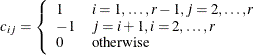
Dunnett-Hsu adjustment: With the first group defined as the control, there are $r-1$ comparisons to be made. Let $\bC =(c_{ij})$ be the $(r-1)\times r$ matrix of contrasts that represents the $r-1$ comparisons; that is,

$\begin{eqnarray*} c_{ij} = \left\{ \begin{array}{ll} 1 & i=1,\ldots ,r-1,j=2,\ldots ,r\\ -1 & j=i+1, i=2,\ldots ,r \\ 0 & \mr{otherwise} \end{array} \right. \end{eqnarray*}$

Let $\bSigma \equiv (\sigma _{ij})$ and $\bR \equiv (r_{ij})$ be covariance and correlation matrices of $\bC \mb{v}$ , respectively; that is,

$\bSigma = \bC \bV \bC ’$

and

$r_{ij}= \frac{\sigma _{ij}}{\sqrt {\sigma _{ii}\sigma _{jj}}}$

The factor-analytic covariance approximation of Hsu (1992) is to find $\lambda _1,\ldots ,\lambda _{r-1}$ such that

$\bR = \bD + \blambda \blambda ’$

where $\bD$ is a diagonal matrix whose jth diagonal element is $1-\lambda _ j$ and $\blambda =(\lambda _1,\ldots ,\lambda _{r-1})’$ . The adjusted p-value is

$p= 1 - \int _{-\infty }^{\infty } \phi (y) \prod _{i=1}^{r-1} \biggl [ \Phi \biggl (\frac{\lambda _ i y + z_{jl}}{\sqrt {1-\lambda _ i^2}}\biggr ) - \Phi \biggl (\frac{\lambda _ i y - z_{jl}}{\sqrt {1-\lambda _ i^2}} \biggr ) \biggr ]dy$

This value can be obtained in a DATA step as

$p=\mr{PROBMC}(\mr{"DUNNETT2"}, z_{ij},.,.,r-1,\lambda _1,\ldots ,\lambda _{r-1}).$
Scheffé adjustment:

$p = \mr{Pr}(\chi ^2_{r-1} > z^2_{jl})$
Šidák adjustment:

$p = 1-\{ 1- \mr{Pr}(\chi ^2_1 > z^2_{jl})\} ^ m$
SMM adjustment:

$p = 1 - [2\Phi (z_{jl}) -1]^ m$

This can also be evaluated in a DATA step as

$p = 1 - \mr{PROBMC}(\mr{"MAXMOD"},z_{jl},.,.,m).$
Tukey adjustment:

$p = 1 - \int _{-\infty }^{\infty } r \phi (y)[\Phi (y) - \Phi (y-\sqrt {2}z_{jl})]^{r-1}dy$

This can be evaluated in a DATA step as

$p = 1 - \mr{PROBMC}(\mr{"RANGE"},\sqrt {2}z_{jl},.,.,r).$

Trend Tests

Trend tests for right-censored data (Klein and Moeschberger, 1997, Section 7.4) can be extended to interval-censored data in a straightforward way. Such tests are specifically designed to detect ordered alternatives as

$H_1\colon S_1(t) \ge S_2(t) \ge \cdots \ge S_ K(t), t\le \tau ,$ with at least one inequality

or

$H_2\colon S_1(t) \le S_2(t) \le \cdots \le S_ K(t), t\le \tau ,$ with at least one inequality

Let $a_1 < a_2 < \cdots < a_ K$ be a sequence of scores associated with the k samples. Let $\mb{U}=(U_1,\ldots ,U_ K)$ be the generalized log-rank statistic and $\mb{V}=(V_{jl})$ be the corresponding covariance matrix of size $K \times K$ as constructed in the section Variance Estimation of the Generalized Log-Rank Statistic. The trend test statistic and its standard error are given by $\sum _{j=1}^ k a_ j U_ j$ and $\sum _{j=1}^ k \sum _{l=1}^ K a_ j a_ l V_{jl}$ , respectively. Under the null hypothesis that there is no trend, the following z-score has, asymptotically, a standard normal distribution: