The SURVEYREG Procedure
- Overview
-
Getting Started

-
SyntaxPROC SURVEYREG StatementBY StatementCLASS StatementCLUSTER StatementCONTRAST StatementDOMAIN StatementEFFECT StatementESTIMATE StatementLSMEANS StatementLSMESTIMATE StatementMODEL StatementOUTPUT StatementREPWEIGHTS StatementSLICE StatementSTORE StatementSTRATA StatementTEST StatementWEIGHT Statement
-
Details
-
Examples
- References
Recall the example in the section Getting Started: SURVEYREG Procedure, which analyzed a stratified simple random sample from a junior high school to examine how household income and the number of children in a household affect students’ average weekly spending for ice cream. You can use the same sample to analyze the average weekly spending among male and female students. Because student gender is unrelated to the design of the sample, this kind of analysis is called domain analysis (subgroup analysis).
The data set follows:
data IceCreamDataDomain;
   input Grade Spending Income Gender$ @@;
   datalines;
7   7  39  M   7   7  38  F   8  12  47  F
9  10  47  M   7   1  34  M   7  10  43  M
7   3  44  M   8  20  60  F   8  19  57  M
7   2  35  M   7   2  36  F   9  15  51  F
8  16  53  F   7   6  37  F   7   6  41  M
7   6  39  M   9  15  50  M   8  17  57  F
8  14  46  M   9   8  41  M   9   8  41  F
9   7  47  F   7   3  39  F   7  12  50  M
7   4  43  M   9  14  46  F   8  18  58  M
9   9  44  F   7   2  37  F   7   1  37  M
7   4  44  M   7  11  42  M   9   8  41  M
8  10  42  M   8  13  46  F   7   2  40  F
9   6  45  F   9  11  45  M   7   2  36  F
7   9  46  F
;
data IceCreamDataDomain;
   set IceCreamDataDomain;
   if Grade=7 then Prob=20/1824;
   if Grade=8 then Prob=9/1025;
   if Grade=9 then Prob=11/1151;
   Weight=1/Prob;
run;
data StudentTotals;
   input Grade _TOTAL_;
   datalines;
7 1824
8 1025
9 1151
;
In the data set IceCreamDataDomain, the variable Grade indicates a student’s grade, which is the stratification variable. The variable Spending contains the dollar amount of each student’s average weekly spending for ice cream. The variable Income specifies the household income, in thousands of dollars. The variable Gender indicates a student’s gender. The sampling weights are created by using the reciprocals of the probabilities of selection.
In the data set StudentTotals, the variable Grade is the stratification variable, and the variable _TOTAL_ contains the total numbers of students in the strata in the survey population.
Suppose that you are now interested in estimating the gender domain means of weekly ice cream spending (that is, the average spending for males and females, respectively). You can use the SURVEYMEANS procedure to produce these domain statistics by using the following statements:
proc surveymeans data=IceCreamDataDomain total=StudentTotals;
   strata Grade;
   var spending;
   domain Gender;
   weight Weight;
run;
Output 98.8.1 shows the estimated spending among male and female students.
Output 98.8.1: Estimated Domain Means
| Domain Statistics in Gender | ||||||
|---|---|---|---|---|---|---|
| Gender | Variable | N | Mean | Std Error of Mean | 95% CL for Mean | |
| F | Spending | 19 | 9.376111 | 1.077927 | 7.19202418 | 11.5601988 |
| M | Spending | 21 | 8.923052 | 1.003423 | 6.88992385 | 10.9561807 |
You can also use PROC SURVEYREG to estimate these domain means. The benefit of this alternative approach is that PROC SURVEYREG provides more tools for additional analysis, such as domain means comparisons in a LSMEANS statement.
Suppose that you want to test whether there is a significant difference for the ice cream spending between male and female students. You can use the following statements to perform the test:
title1 'Ice Cream Spending Analysis';
title2 'Compare Domain Statistics';
proc surveyreg data=IceCreamDataDomain total=StudentTotals;
   strata Grade;
   class Gender;
   model Spending = Gender / vadjust=none;
   lsmeans Gender / diff;
   weight Weight;
run;
The variable Gender is used as a model effect. The VADJUST=NONE option is used to produce variance estimates for domain means that are identical to those produced by PROC SURVEYMEANS. The
LSMEANS statement requests that PROC SURVEYREG estimate the average spending in each gender group. The DIFF option requests that the procedure compute the difference among domain means.
Output 98.8.2 displays the estimated weekly spending on ice cream among male and female students, respectively, and their standard errors. Female students spend $9.38 per week on average, and male students spend $8.92 per week on average. These domain means, including their standard errors, are identical to those in Output 98.8.1 which are produced by PROC SURVEYMEANS.
Output 98.8.2: Domain Means between Gender
| Ice Cream Spending Analysis |
| Compare Domain Statistics |
| Gender Least Squares Means | |||||
|---|---|---|---|---|---|
| Gender | Estimate | Standard Error | DF | t Value | Pr > |t| |
| F | 9.3761 | 1.0779 | 37 | 8.70 | <.0001 |
| M | 8.9231 | 1.0034 | 37 | 8.89 | <.0001 |
Output 98.8.3 shows the estimated difference for weekly ice scream spending between the two gender groups. The female students spend $0.45 more than male students on average, and the difference is not statistically significant based on the t test.
Output 98.8.3: Domain Means Comparison
| Differences of Gender Least Squares Means | ||||||
|---|---|---|---|---|---|---|
| Gender | _Gender | Estimate | Standard Error | DF | t Value | Pr > |t| |
| F | M | 0.4531 | 1.7828 | 37 | 0.25 | 0.8008 |
If you want to investigate whether there is any significant difference in ice cream spending among grades, you can use the following similar statements to compare:
ods graphics on;
title1 'Ice Cream Spending Analysis';
title2 'Compare Domain Statistics';
proc surveyreg data=IceCreamDataDomain total=StudentTotals;
   strata Grade;
   class Grade;
   model Spending = Grade / vadjust=none;
   lsmeans Grade / diff plots=(diff meanplot(cl));
   weight Weight;
run;
ods graphics off;
The Grade is specified in the CLASS statement to be used as an effect in the MODEL statement. The DIFF option in the LSMEANS statement requests that the procedure compute the difference among the domain means for the effect Grade. The ODS GRAPHICS statement enables ODS to create graphics. The PLOTS=(DIFF MEANPLOT(CL)) option requests two graphics: the domain means plot MeanPlot and their pairwise difference plot DiffPlot. The CL suboption requests the MeanPlot to display confidence. For information about ODS Graphics, see Chapter 21: Statistical Graphics Using ODS.
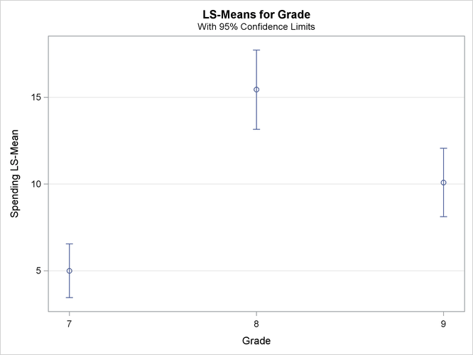
Output 98.8.4 shows the estimated weekly spending on ice cream for students within each grade. Students in Grade 7 spend the least, only $5.00 per week. Students in Grade 8 spend the most, $15.44 per week. Students in Grade 9 spend a little less at $10.09 per week.
Output 98.8.4: Domain Means among Grades
| Ice Cream Spending Analysis |
| Compare Domain Statistics |
| Grade Least Squares Means | |||||
|---|---|---|---|---|---|
| Grade | Estimate | Standard Error | DF | t Value | Pr > |t| |
| 7 | 5.0000 | 0.7636 | 37 | 6.55 | <.0001 |
| 8 | 15.4444 | 1.1268 | 37 | 13.71 | <.0001 |
| 9 | 10.0909 | 0.9719 | 37 | 10.38 | <.0001 |
Output 98.8.5 plots the weekly spending results that are shown in Output 98.8.4.
Output 98.8.6 displays pairwise comparisons for weekly ice scream spending among grades. All the differences are significant based on t tests.
Output 98.8.6: Domain Means Comparison
| Differences of Grade Least Squares Means | ||||||
|---|---|---|---|---|---|---|
| Grade | _Grade | Estimate | Standard Error | DF | t Value | Pr > |t| |
| 7 | 8 | -10.4444 | 1.3611 | 37 | -7.67 | <.0001 |
| 7 | 9 | -5.0909 | 1.2360 | 37 | -4.12 | 0.0002 |
| 8 | 9 | 5.3535 | 1.4880 | 37 | 3.60 | 0.0009 |
Output 98.8.7 plots the comparisons that are shown in Output 98.8.6.
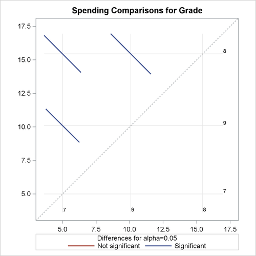
In Output 98.8.7, the spending for each grade is shown in the background grid on both axes. Comparisons for each pair of domain means are shown by colored bars at intersections of these grids. The length of each bar represents the width of the confidence intervals for the corresponding difference between domain means. The significance of these pairwise comparisons are indicated in the plot by whether these bars cross the 45-degree background dash-line across the plot. Since none of the three bars cross the dash-line, all pairwise comparisons are significant, as shown in Output 98.8.6.