The SURVEYREG Procedure
- Overview
-
Getting Started

-
SyntaxPROC SURVEYREG StatementBY StatementCLASS StatementCLUSTER StatementCONTRAST StatementDOMAIN StatementEFFECT StatementESTIMATE StatementLSMEANS StatementLSMESTIMATE StatementMODEL StatementOUTPUT StatementREPWEIGHTS StatementSLICE StatementSTORE StatementSTRATA StatementTEST StatementWEIGHT Statement
-
Details
-
Examples
- References
This example investigates the relationship between the labor force participation rate (LFPR) of women in 1968 and 1972 in
large cities in the United States. A simple random sample of 19 cities is drawn from a total of 200 cities. For each selected
city, the LFPRs are recorded and saved in a SAS data set Labor. In the following DATA step, LFPR in 1972 is contained in the variable LFPR1972, and the LFPR in 1968 is identified by the variable LFPR1968:
data Labor;
   input City $ 1-16 LFPR1972 LFPR1968;
   datalines;
New York        .45     .42
Los Angeles     .50     .50
Chicago         .52     .52
Philadelphia    .45     .45
Detroit         .46     .43
San Francisco   .55     .55
Boston          .60     .45
Pittsburgh      .49     .34
St. Louis       .35     .45
Connecticut     .55     .54
Washington D.C. .52     .42
Cincinnati      .53     .51
Baltimore       .57     .49
Newark          .53     .54
Minn/St. Paul   .59     .50
Buffalo         .64     .58
Houston         .50     .49
Patterson       .57     .56
Dallas          .64     .63
;
Assume that the LFPRs in 1968 and 1972 have a linear relationship, as shown in the following model:
You can use PROC SURVEYREG to obtain the estimated regression coefficients and estimated standard errors of the regression coefficients. The following statements perform the regression analysis:
ods graphics on;
title 'Study of Labor Force Participation Rates of Women';
proc surveyreg data=Labor total=200;
   model LFPR1972 = LFPR1968;
run;
ods graphics off;
Here, the TOTAL=200 option specifies the finite population total from which the simple random sample of 19 cities is drawn. You can specify the same information by using the sampling rate option RATE=0.095 (19/200=.095).
Output 98.1.1 summarizes the data information and the fit information.
Output 98.1.1: Summary of Regression Using Simple Random Sampling
| Study of Labor Force Participation Rates of Women |
| Data Summary | |
|---|---|
| Number of Observations | 19 |
| Mean of LFPR1972 | 0.52684 |
| Sum of LFPR1972 | 10.01000 |
| Fit Statistics | |
|---|---|
| R-Square | 0.3970 |
| Root MSE | 0.05657 |
| Denominator DF | 18 |
Output 98.1.2 presents the significance tests for the model effects and estimated regression coefficients. The F tests and t tests for the effects in the model are also presented in these tables.
Output 98.1.2: Regression Coefficient Estimates
| Tests of Model Effects | |||
|---|---|---|---|
| Effect | Num DF | F Value | Pr > F |
| Model | 1 | 13.84 | 0.0016 |
| Intercept | 1 | 4.63 | 0.0452 |
| LFPR1968 | 1 | 13.84 | 0.0016 |
| Note: | The denominator degrees of freedom for the F tests is 18. |
| Estimated Regression Coefficients | ||||
|---|---|---|---|---|
| Parameter | Estimate | Standard Error | t Value | Pr > |t| |
| Intercept | 0.20331056 | 0.09444296 | 2.15 | 0.0452 |
| LFPR1968 | 0.65604048 | 0.17635810 | 3.72 | 0.0016 |
| Note: | The denominator degrees of freedom for the t tests is 18. |
From the regression performed by PROC SURVEYREG, you obtain a positive estimated slope for the linear relationship between
the LFPR in 1968 and the LFPR in 1972. The regression coefficients are all significant at the 5% level. The effects Intercept and LFPR1968 are significant in the model at the 5% level. In this example, the F test for the overall model without intercept is the same as the effect LFPR1968.
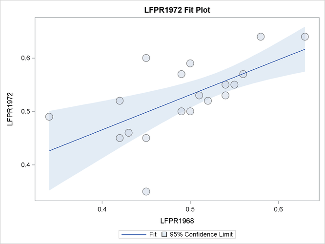
When ODS graphics is enabled and you have only one regressor in the model, PROC SURVEYREG displays a plot of the model fitting, which is shown in Output 98.1.3.