The MULTTEST Procedure

An experiment was performed using Affymetrix® gene chips on the CD4 lymphocyte white blood cells of patients with and without a hereditary allergy (atopy) and possibly
with asthma. The Asthma-Atopy microarray data set and analysis are discussed in Gibson and Wolfinger (2004): a one-way ANOVA model of the log2mas5 variable (![]() summary statistics) is fit against a classification variable
summary statistics) is fit against a classification variable trt describing different asthma-atopy combinations in the patients, and the least squares means of the trt variable are computed.
For this example, a 1% random sample of least squares means having p-values exceeding 1E–6 is taken. The resulting data are recorded in the test data set, where the Probe_Set_ID variable identifies the probe and the Probt variable contains the p-values for the m = 121 tests, as follows:
data test;
   length Probe_Set_ID $9.;
   input Probe_Set_ID $ Probt @@;
   datalines;
200973_s_ .963316  201059_at .462754  201563_at .000409  201733_at .000819
201951_at .000252  202944_at .106550  203107_x_ .040396  203372_s_ .010911
203469_s_ .987234  203641_s_ .019296  203795_s_ .002276  204055_s_ .002328
205020_s_ .008628  205199_at .608129  205373_at .005209  205384_at .742381
205428_s_ .870533  205653_at .621671  205686_s_ .396440  205760_s_ .000002
206032_at .024661  206159_at .997627  206223_at .003702  206398_s_ .191682
206623_at .010030  206852_at .000004  207072_at .000214  207371_at .000013
207789_s_ .023623  207861_at .000002  207897_at .000007  208022_s_ .251999
208086_s_ .000361  208406_s_ .040182  208464_at .161468  209055_s_ .529824
209125_at .142276  209369_at .240079  209748_at .071750  209894_at .000042
209906_at .223282  210130_s_ .192187  210199_at .101623  210477_x_ .300038
210491_at .000078  210531_at .000784  210734_x_ .202931  210755_at .009644
210782_x_ .000011  211320_s_ .022896  211329_x_ .486869  211362_s_ .881798
211369_at .000030  211399_at .000008  211572_s_ .269788  211647_x_ .001301
213072_at .005019  213143_at .008711  213238_at .004824  213391_at .316133
213468_at .000172  213636_at .097133  213823_at .001678  213854_at .001921
213976_at .000299  214006_s_ .014616  214063_s_ .000361  214407_x_ .609880
214445_at .000009  214570_x_ .000002  214648_at .001255  214684_at .288156
214991_s_ .006695  215012_at .000499  215117_at .000136  215201_at .045235
215304_at .000816  215342_s_ .973786  215392_at .112937  215557_at .000007
215608_at .006204  215935_at .000027  215980_s_ .037382  216010_x_ .000354
216051_x_ .000003  216086_at .002310  216092_s_ .000056  216511_s_ .294776
216733_s_ .004823  216747_at .002902  216874_at .000117  216969_s_ .001614
217133_x_ .056851  217198_x_ .169196  217557_s_ .002966  217738_at .000005
218601_at .023817  218818_at .027554  219302_s_ .000039  219441_s_ .000172
219574_at .193737  219612_s_ .000075  219697_at .046476  219700_at .003049
219945_at .000066  219964_at .000684  220234_at .130064  220473_s_ .000017
220575_at .030223  220633_s_ .058460  220925_at .252465  221256_s_ .721731
221314_at .002307  221589_s_ .001810  221995_s_ .350859  222071_s_ .000062
222113_s_ .000023  222208_s_ .100961  222303_at .049265  37226_at  .000749
60474_at  .000423
run;
The following statements adjust the p-values in the test data set by using the adaptive adjustments (ADAPTIVEHOLM, ADAPTIVEHOCHBERG, ADAPTIVEFDR, and PFDR), which require an estimate of the number of true null hypotheses (![]() ) or proportion of true null hypotheses (
) or proportion of true null hypotheses (![]() ). This example illustrates some of the features and graphics for computing and evaluating these estimates. The NOPVALUE option is specified to suppress the display of the “p-Values” table.
). This example illustrates some of the features and graphics for computing and evaluating these estimates. The NOPVALUE option is specified to suppress the display of the “p-Values” table.
ods graphics on;
proc multtest inpvalues(Probt)=test plots=all seed=518498000
              aholm ahoc afdr pfdr(positive) nopvalue;
   id Probe_Set_ID;
run;
ods graphics off;
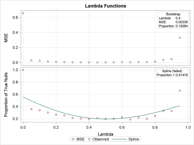
Output 65.6.1 lists the requested p-value adjustments, along with the selected value of the “Lambda” tuning parameter and the seed (specified with the SEED= option) used in the bootstrap method of estimating the number of true null hypotheses. The “Lambda Values” table lists the estimated number of true nulls for each value of ![]() , where you can see that the minimum MSE (0.002315) occurs at
, where you can see that the minimum MSE (0.002315) occurs at ![]() . Output 65.6.2 shows that the SPLINE method failed due to a large slope at
. Output 65.6.2 shows that the SPLINE method failed due to a large slope at ![]() , so the bootstrap method is used and the MSE plot is displayed.
, so the bootstrap method is used and the MSE plot is displayed.
Output 65.6.1: p and Lambda Values
| P-Value Adjustment Information | |
|---|---|
| P-Value Adjustment | Adaptive Holm |
| P-Value Adjustment | Adaptive Hochberg |
| P-Value Adjustment | Adaptive FDR |
| P-Value Adjustment | pFDR Q-Value |
| Lambda | 0.4 |
| Seed | 518498000 |
| Lambda Values | |||
|---|---|---|---|
| Lambda | MSE | NTrueNull Observed |
NTrueNull Spline |
| 0 | 0.657880 | 121.000000 | 67.318707 |
| 0.050000 | 0.030212 | 43.157895 | 59.812885 |
| 0.100000 | 0.024897 | 41.111111 | 52.636271 |
| 0.150000 | 0.014904 | 36.470588 | 46.033846 |
| 0.200000 | 0.008580 | 32.500000 | 40.172642 |
| 0.250000 | 0.006476 | 30.666667 | 35.157768 |
| 0.300000 | 0.002719 | 25.714286 | 31.046105 |
| 0.350000 | 0.002471 | 24.615385 | 27.861153 |
| 0.400000 | 0.002378 | 23.333333 | 25.595089 |
| 0.450000 | 0.003285 | 25.454545 | 24.217908 |
| 0.500000 | 0.003036 | 24.000000 | 23.687690 |
| 0.550000 | 0.003567 | 24.444444 | 23.965745 |
| 0.600000 | 0.005813 | 27.500000 | 25.016579 |
| 0.650000 | 0.004118 | 22.857143 | 26.809774 |
| 0.700000 | 0.006647 | 26.666667 | 29.321876 |
| 0.750000 | 0.006260 | 24.000000 | 32.512203 |
| 0.800000 | 0.013242 | 30.000000 | 36.315191 |
| 0.850000 | 0.037624 | 40.000000 | 40.618909 |
| 0.900000 | 0.046906 | 40.000000 | 45.274355 |
| 0.950000 | 0.332183 | 80.000000 | 50.117369 |
Output 65.6.3 also shows that the bootstrap estimate is used for the PFDR adjustment. The other adjustments have different default methods for estimating the number of true nulls.
Output 65.6.3: Adjustments and Their Default Estimation Method
| Estimated Number of True Null Hypotheses | |||
|---|---|---|---|
| P-Value Adjustment | Method | Estimate | Proportion |
| Adaptive Holm | Decreased Slope | 26 | 0.21488 |
| Adaptive Hochberg | Decreased Slope | 26 | 0.21488 |
| Adaptive FDR | Lowest Slope | 43 | 0.35537 |
| Positive FDR | Bootstrap | 23.3333 | 0.19284 |
Output 65.6.4 displays the estimated number of true nulls ![]() against a uniform probability plot of the unadjusted p-values (if the p-values are distributed uniformly, the points on the plot will all lie on a straight line). According to Schweder and Spjøtvoll
(1982) and Hochberg and Benjamini (1990), the points on the left side of the plot should be approximately linear with slope
against a uniform probability plot of the unadjusted p-values (if the p-values are distributed uniformly, the points on the plot will all lie on a straight line). According to Schweder and Spjøtvoll
(1982) and Hochberg and Benjamini (1990), the points on the left side of the plot should be approximately linear with slope ![]() , so you can use this plot to evaluate whether your estimate of
, so you can use this plot to evaluate whether your estimate of ![]() seems reasonable.
seems reasonable.

The NTRUENULL= option provides several methods for estimating the number of true null hypotheses; the following table displays each method and its estimate for this example:
|
NTRUENULL= |
Estimate |
|---|---|
|
BOOTSTRAP |
23.3 |
|
DECREASESLOPE |
26 |
|
KSTEST |
35 |
|
LEASTSQUARES |
28 |
|
LOWESTSLOPE |
43 |
|
MEANDIFF |
42 |
|
SPLINE |
50.1 |
Another method of estimating the number of true null hypotheses fits a finite mixture model (mixing a uniform with a beta) to the distribution of the unadjusted p-values (Allison et al., 2002). Osborne (2006) provides the following PROC NLMIXED statements to fit this model:
proc nlmixed data=test;
   parameters pi0=0.5 a=.1 b=.1;
   pi1= 1-pi0;
   bounds 0 <= pi0 <= 1;
   loglikelihood= log(pi0+pi1*pdf('beta',Probt,a,b));
   model Probt ~ general(loglikelihood);
run;
You might have to change the initial parameter values in the PARAMETERS statement to achieve convergence; see Chapter 68: The NLMIXED Procedure, for more information. This mixture model estimates ![]() , meaning that the distribution of p-values is completely specified by a single beta distribution. If the estimate were, say,
, meaning that the distribution of p-values is completely specified by a single beta distribution. If the estimate were, say, ![]() , you could then specify it as follows:
, you could then specify it as follows:
proc multtest inpvalues(Probt)=test ptruenull=0.10
              aholm ahoc afdr pfdr(positive) nopvalue;
   id Probe_Set_ID;
run;
A plot of the unadjusted and adjusted p-values for each test is also produced. Due to the large number of tests and adjustments, the plot is not very informative and is not displayed here.
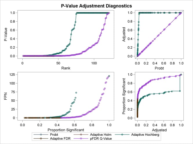
The top two plots in Output 65.6.5 show how the adjusted values compare with each other and the unadjusted p-values. The PFDR and AFDR adjustments are eventually smaller than the unadjusted p-values since they control the false discovery rate. The adaptive Holm and Hochberg adjustments are almost identical, so the adaptive Holm values are mostly obscured in all four plots. The plot of the Proportion Significant versus the Adjusted p-values tells you how many of the tests are significant for each cutoff, while the plot of the number of false positives (FPN) versus the Proportion Significant tells you how many false positives you can expect for that cutoff.
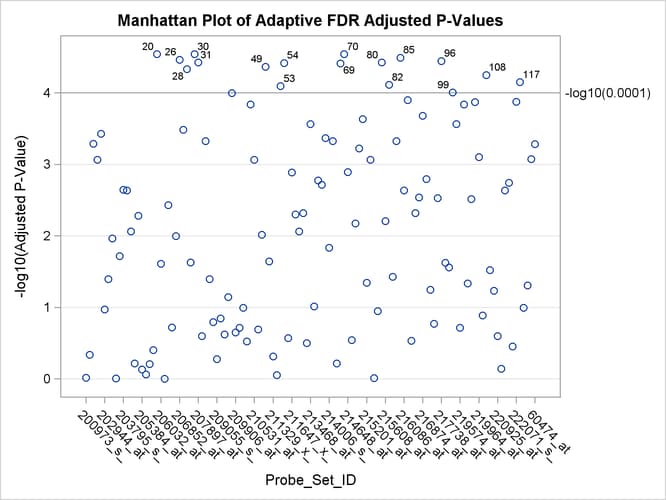
A Manhattan plot displays –log![]() of the adjusted p-values, so the most significant tests stand out at the top of the plot. The default plot is not displayed here. The following
statements create a Manhattan plot of the adaptive FDR p-values, with the most significant tests labeled with their observation number. The ID values are displayed on the X axis,
and the VREF= option specifies the significance level. This plot is typically created with many more p-values, and special ODS Graphics options such as the LABELMAX= option might be required to display the graph. If memory usage
is an issue, you might want to store your p-values and use the SGPLOT procedure to create a similar graph.
of the adjusted p-values, so the most significant tests stand out at the top of the plot. The default plot is not displayed here. The following
statements create a Manhattan plot of the adaptive FDR p-values, with the most significant tests labeled with their observation number. The ID values are displayed on the X axis,
and the VREF= option specifies the significance level. This plot is typically created with many more p-values, and special ODS Graphics options such as the LABELMAX= option might be required to display the graph. If memory usage
is an issue, you might want to store your p-values and use the SGPLOT procedure to create a similar graph.
ods graphics on / labelmax=1000;
proc multtest inpvalues(Probt)=test afdr nopvalue
   plots=Manhattan(label=obs vref=0.0001);
   id Probe_Set_ID;
run;
ods graphics off;
If you have a lot of tests, the “Raw and Adjusted p-Values” and “P-Value Adjustment Diagnostics” plots can be more informative if you suppress some of the tests. In the following statements, the SIGONLY=0.001 option selects tests with adjusted p-values < 0.001 for display. Output 65.6.7 displays tests with their “significant” adjusted p-values:
ods graphics on;
proc multtest inpvalues(Probt)=test plots(sigonly=0.001)=PByTest
              aholm ahoc afdr pfdr(positive) nopvalue;
run;
ods graphics off;
