p-Value Adjustments :: SAS/STAT(R) 13.1 User's Guide

p-Value Adjustments

Subsections:

Familywise Error Rate Controlling Adjustments
False Discovery Rate Controlling Adjustments

Suppose you test m null hypotheses, $H_{01},\ldots ,H_{0m}$ , and obtain the p-values $p_1,\ldots ,p_ m$ . Denote the ordered p-values as $p_{(1)}\le \ldots \le p_{(m)}$ and order the tests appropriately: $H_{0(1)},\ldots ,H_{0(m)}$ . Suppose you know $m_0$ of the null hypotheses are true and $m_1=m-m_0$ are false. Let R indicate the number of null hypotheses rejected by the tests, where V of these are incorrectly rejected (that is, V tests are Type I errors) and $R-V$ are correctly rejected (so $m_1-R+V$ tests are Type II errors). This information is summarized in the following table:

	Null is Rejected	Null is Not Rejected	Total
Null is True	V	m $_0$ – V	m $_0$
Null is False	R – V	m $_1$ – R + V	m $_1$
Total	R	m – R	m

The familywise error rate (FWE) is the overall Type I error rate for all the comparisons (possibly under some restrictions); that is, it is the maximum probability of incorrectly rejecting one or more null hypotheses:

$\mbox{FWE} = \Pr (V > 0)$

The FWE is also known as the maximum experimentwise error rate (MEER), as discussed in the section Pairwise Comparisons in Chapter 44: The GLM Procedure.

The false discovery rate (FDR) is the expected proportion of incorrectly rejected hypotheses among all rejected hypotheses:

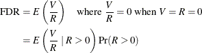
$\begin{align*} \hbox{FDR} & = E\left(\frac{V}{R}\right) \quad \mbox{where } \frac{V}{R}=0 \mbox{ when } V=R=0 \\ & = E\left(\frac{V}{R}~ |~ R>0\right)\Pr (R>0) \end{align*}$

Under the overall null hypothesis (all the null hypotheses are true), the FDR=FWE since V = R gives $E\left(\frac{V}{R}\right)=1\times \Pr \left(\frac{V}{R} = 1\right)= \Pr (V > 0)$ . Otherwise, FDR is always less than FWE, and an FDR-controlling adjustment also controls the FWE. Another definition used is the positive false discovery rate:

$\hbox{pFDR} = E\left(\frac{V}{R}~ |~ R>0\right)$

The p-value adjustment methods discussed in the following sections attempt to correct the raw p-values while controlling either the FWE or the FDR. Note that the methods might impose some restrictions in order to achieve this; restrictions are discussed along with the methods in the following sections. Discussions and comparisons of some of these methods are given in Dmitrienko et al. (2005), Dudoit, Shaffer, and Boldrick (2003), Westfall et al. (1999), and Brown and Russell (1997).

Familywise Error Rate Controlling Adjustments

PROC MULTTEST provides several p-value adjustments to control the familywise error rate. Single-step adjustment methods are computed without reference to the other hypothesis tests under consideration. The available single-step methods are the Bonferroni and Šidák adjustments, which are simple functions of the raw p-values that try to distribute the significance level $\alpha$ across all the tests, and the bootstrap and permutation resampling adjustments, which require the raw data. The Bonferroni and Šidák methods are calculated from the permutation distributions when exact permutation tests are used with the CA or Peto test.

Stepwise tests, or sequentially rejective tests, order the hypotheses in step-up (least significant to most significant) or step-down fashion, then sequentially determine acceptance or rejection of the nulls. These tests are more powerful than the single-step tests, and they do not always require you to perform every test. However, PROC MULTTEST still adjusts every p-value. PROC MULTTEST provides the following stepwise p-value adjustments: step-down Bonferroni (Holm), step-down Šidák, step-down bootstrap and permutation resampling, Hochberg’s (1988) step-up, Hommel’s (1988), Fisher’s combination method, and the Stouffer-Liptak combination method. Adaptive versions of Holm’s step-down Bonferroni and Hochberg’s step-up Bonferroni methods, which require an estimate of the number of true null hypotheses, are also available.

Liu (1996) shows that all single-step and stepwise tests based on marginal p-values can be used to construct a closed test (Marcus, Peritz, and Gabriel, 1976; Dmitrienko et al., 2005). Closed testing methods not only control the familywise error rate at size $\alpha$ , but are also more powerful than the tests on which they are based. Westfall and Wolfinger (2000) note that several of the methods available in PROC MULTTEST are closed—namely, the step-down methods, Hommel’s method, and Fisher’s combination; see that reference for conditions and exceptions.

All methods except the resampling methods are calculated by simple functions of the raw p-values or marginal permutation distributions; the permutation and bootstrap adjustments require the raw data. Because the resampling techniques incorporate distributional and correlational structures, they tend to be less conservative than the other methods.

When a resampling (bootstrap or permutation) method is used with only one test, the adjusted p-value is the bootstrap or permutation p-value for that test, with no adjustment for multiplicity, as described by Westfall and Soper (1994).

Bonferroni

The Bonferroni p-value for test $i, i=1,\ldots ,m$ is simply $\tilde{p}_ i=m p_ i$ . If the adjusted p-value exceeds 1, it is set to 1. The Bonferroni test is conservative but always controls the familywise error rate.

If the unadjusted p-values are computed by using exact permutation distributions, then the Bonferroni adjustment for $p_ i$ is $\tilde{p}_ i=p_1^*+ \cdots + p_ m^*$ , where $p_ j^*$ is the largest p-value from the permutation distribution of test j satisfying $p_ j^* \le p_ i$ , or 0 if all permutational p-values of test j are greater than $p_ i$ . These adjustments are much less conservative than the ordinary Bonferroni adjustments because they incorporate the discrete distributional characteristics. However, they remain conservative in that they do not incorporate correlation structures between multiple contrasts and multiple variables (Westfall and Wolfinger, 1997).

Šidák

A technique slightly less conservative than Bonferroni is the Šidák p-value (Šidák, 1967), which is $\tilde{p}_ i=1 - (1 - p_ i)^ m$ . It is exact when all of the p-values are uniformly distributed and independent, and it is conservative when the test statistics satisfy the positive orthant dependence condition (Holland and Copenhaver, 1987).

If the unadjusted p-values are computed by using exact permutation distributions, then the Šidák adjustment for $p_ i$ is $\tilde{p}_ i=1-(1-p_1^*) \cdots (1- p_ m^*)$ , where the $p_ j^*$ are as described previously. These adjustments are less conservative than the corresponding Bonferroni adjustments, but they do not incorporate correlation structures between multiple contrasts and multiple variables (Westfall and Wolfinger, 1997).

Bootstrap

The bootstrap method creates pseudo-data sets by sampling observations with replacement from each within-stratum pool of observations. An entire data set is thus created, and p-values for all tests are computed on this pseudo-data set. A counter records whether the minimum p-value from the pseudo-data set is less than or equal to the actual p-value for each base test. (If there are m tests, then there are m such counters.) This process is repeated a large number of times, and the proportion of resampled data sets where the minimum pseudo-p-value is less than or equal to an actual p-value is the adjusted p-value reported by PROC MULTTEST. The algorithms are described in Westfall and Young (1993).

In the case of continuous data, the pooling of the groups is not likely to re-create the shape of the null hypothesis distribution, since the pooled data are likely to be multimodal. For this reason, PROC MULTTEST automatically mean-centers all continuous variables prior to resampling. Such mean-centering is akin to resampling residuals in a regression analysis, as discussed by Freedman (1981). You can specify the NOCENTER option if you do not want to center the data.

The bootstrap method implicitly incorporates all sources of correlation, from both the multiple contrasts and the multivariate structure. The adjusted p-values incorporate all correlations and distributional characteristics. This method always provides weak control of the familywise error rate, and it provides strong control when the subset pivotality condition holds; that is, for any subset of the null hypotheses, the joint distribution of the p-values for the subset is identical to that under the complete null (Westfall and Young, 1993).

Permutation

The permutation-style-adjusted p-values are computed in identical fashion as the bootstrap-adjusted p-values, with the exception that the within-stratum resampling is performed without replacement instead of with replacement. This produces a rerandomization analysis such as in Brown and Fears (1981) and Heyse and Rom (1988). In the spirit of rerandomization analyses, the continuous variables are not centered prior to resampling. This default can be overridden by using the CENTER option.

The permutation method implicitly incorporates all sources of correlation, from both the multiple contrasts and the multivariate structure. The adjusted p-values incorporate all correlations and distributional characteristics. This method always provides weak control of the familywise error rate, and it provides strong control of the familywise error rate under the subset pivotality condition, as described in the preceding section.

Step-Down Methods

Step-down testing is available for the Bonferroni, Šidák, bootstrap, and permutation methods. The benefit of using step-down methods is that the tests are made more powerful (smaller adjusted p-values) while, in most cases, maintaining strong control of the familywise error rate. The step-down method was pioneered by Holm (1979) and further developed by Shaffer (1986), Holland and Copenhaver (1987), and Hochberg and Tamhane (1987).

The Bonferroni step-down (Holm) p-values $\tilde{p}_{(1)},\ldots ,\tilde{p}_{(m)}$ are obtained from

$\begin{equation*} \tilde{p}_{(i)} = \begin{cases} m p_{(1)} & \mbox{for } i=1 \\ \max \left( \tilde{p}_{(i-1)} , (m-i+1) p_{(i)} \right) & \mbox{for } i=2,\ldots ,m \end{cases}\end{equation*}$

As always, if any adjusted p-value exceeds 1, it is set to 1.

The Šidák step-down p-values are determined similarly:

$\begin{equation*} \tilde{p}_{(i)} = \begin{cases} 1 - (1 - p_{(1)})^ m & \mbox{for } i=1 \\ \max \left( \tilde{p}_{(i-1)} , 1 - (1 - p_{(i)})^{m-i+1} \right) & \mbox{for } i=2,\ldots ,m \end{cases}\end{equation*}$

Step-down Bonferroni adjustments that use exact tests are defined as

$\begin{equation*} \tilde{p}_{(i)} = \begin{cases} p_{(1)}^*+ \cdots + p_{(m)}^* & \mbox{for } i=1 \\ \max \left( \tilde{p}_{(i-1)} , p_{(i)}^*+ \cdots + p_{(m)}^*, \right) & \mbox{for } i=2,\ldots ,m \end{cases}\end{equation*}$

where the $p_ j^*$ are defined as before. Note that $p_ j^*$ is taken from the permutation distribution corresponding to the jth-smallest unadjusted p-value. Also, any $\tilde{p}_ j$ greater than 1.0 is reduced to 1.0.

Step-down Šidák adjustments for exact tests are defined analogously by substituting $1-(1-p_{(j)}^*)\cdots (1-p_{(m)}^*)$ for $p_{(j)}^* + \cdots + p_{(m)}^*$ .

The resampling-style step-down methods are analogous to the preceding step-down methods; the most extreme p-value is adjusted according to all m tests, the second-most extreme p-value is adjusted according to (m – 1) tests, and so on. The difference is that all correlational and distributional characteristics are incorporated when you use resampling methods. More specifically, assuming the same ordering of p-values as discussed previously, the resampling-style step-down-adjusted p-value for test i is the probability that the minimum pseudo-p-value of tests $i,\ldots ,m$ is less than or equal to $p_ i$ .

This probability is evaluated by using Monte Carlo simulation, as are the previously described resampling-style-adjusted p-values. In fact, the computations for step-down-adjusted p-values are essentially no more time-consuming than the computations for the non-step-down-adjusted p-values. After Monte Carlo, the step-down-adjusted p-values are corrected to ensure monotonicity; this correction leaves the first adjusted p-values alone, then corrects the remaining ones as needed. The step-down method approximately controls the familywise error rate, and it is described in more detail by Westfall and Young (1993), Westfall et al. (1999), and Westfall and Wolfinger (2000).

Hommel

Hommel’s (1988) method is a closed testing procedure based on Simes’ test (Simes, 1986). The Simes p-value for a joint test of any set of S hypotheses with p-values $p_{(1)} \leq p_{(2)} \leq \ldots \leq p_{(S)}$ is $\mbox{min}((S/1)p_{(1)},(S/2)p_{(2)},\ldots ,(S/S)p_{(S)})$ . The Hommel-adjusted p-value for test j is the maximum of all such Simes p-values, taken over all joint tests that include j as one of their components.

Hochberg-adjusted p-values are always as large or larger than Hommel-adjusted p-values. Sarkar and Chang (1997) shows that Simes’ method is valid under independent or positively dependent p-values, so Hommel’s and Hochberg’s methods are also valid in such cases by the closure principle.

Hochberg

Assuming p-values are independent and uniformly distributed under their respective null hypotheses, Hochberg (1988) demonstrates that Holm’s step-down adjustments control the familywise error rate even when calculated in step-up fashion. Since the adjusted p-values are uniformly smaller for Hochberg’s method than for Holm’s method, the Hochberg method is more powerful. However, this improved power comes at the cost of having to make the assumption of independence. Hochberg’s method can be derived from Hommel’s (Liu, 1996), and is thus also derived from Simes’ test (Simes, 1986).

Hochberg-adjusted p-values are always as large or larger than Hommel-adjusted p-values. Sarkar and Chang (1997) showed that Simes’ method is valid under independent or positively dependent p-values, so Hommel’s and Hochberg’s methods are also valid in such cases by the closure principle.

The Hochberg-adjusted p-values are defined in reverse order of the step-down Bonferroni:

$\begin{equation*} \tilde{p}_{(i)} = \begin{cases} p_{(m)} & \mbox{for } i=m \\ \min \left( \tilde{p}_{(i+1)} , (m-i+1) p_{(i)} \right) & \mbox{for } i=m-1,\ldots ,1 \end{cases}\end{equation*}$

Fisher Combination

The FISHER_C option requests adjusted p-values by using closed tests, based on the idea of Fisher’s combination test. The Fisher combination test for a joint test of any set of S hypotheses with p-values uses the chi-square statistic $\chi ^2 = -2 \sum \log (p_ i)$ , with 2S degrees of freedom. The FISHER_C adjusted p-value for test j is the maximum of all p-values for the combination tests, taken over all joint tests that include j as one of their components. Independence of p-values is required for the validity of this method.

Stouffer-Liptak Combination

The STOUFFER option requests adjusted p-values by using closed tests, based on the Stouffer-Liptak combination test. The Stouffer combination joint test of any set of S one-sided hypotheses with p-values, $p_1, \ldots , p_ S$ , yields the p-value, $1-\Phi \left(\frac{1}{\sqrt {S}}\sum _ i\Phi ^{-1}(1-p_ i)\right)$ . The STOUFFER adjusted p-value for test j is the maximum of all p-values for the combination tests, taken over all joint tests that include j as one of their components.

Independence of the one-sided p-values is required for the validity of this method. Westfall (2005) shows that the Stouffer-Liptak adjustment might have more power than the Fisher combination and Simes’ adjustments when the test results reinforce each other.

Adaptive Adjustments

Adaptive adjustments modify the FWE- and FDR-controlling procedures by taking an estimate of the number ${m}_0$ or proportion ${\pi }_0$ of true null hypotheses into account. The adjusted p-values for Holm’s and Hochberg’s methods involve the number of unadjusted p-values larger than ${(i)}$ , $m-i+1$ . So the minimal significance level at which the ith ordered p-value is rejected implies that the number of true null hypotheses is $m-i+1$ . However, if you know $m_0$ , then you can replace $m-i+1$ with $\min (m_0,m-i+1)$ , thereby obtaining more power while maintaining the original $\alpha$ -level significance.

Since $m_0$ is unknown, there are several methods used to estimate the value—see the NTRUENULL= option for more information. The estimation method described by Hochberg and Benjamini (1990) considers the graph of $1-p_{(i)}$ versus i, where the $p_{(i)}$ are the ordered p-values of your tests. See Output 65.6.4 for an example. If all null hypotheses are actually true ( $m_0=m$ ), then the p-values behave like a sample from a uniform distribution and this graph should be a straight line through the origin. However, if points in the upper-right corner of this plot do not follow the initial trend, then some of these null hypotheses are probably false and $0<m_0<m$ .

The ADAPTIVEHOLM option uses this estimate of ${m}_0$ to adjust the step-up Bonferroni method while the ADAPTIVEHOCHBERG option adjusts the step-down Bonferroni method. Both of these methods are due to Hochberg and Benjamini (1990). When $m_0$ is known, these procedures control the familywise error rate in the same manner as their nonadaptive versions but with more power; however, since $m_0$ must be estimated, the FWE control is only approximate. The ADAPTIVEFDR and PFDR options also use $\hat{m}_0$ , and are described in the following section.

The adjusted p-values for the ADAPTIVEHOLM method are computed by

$\begin{equation*} \tilde{p}_{(i)} = \begin{cases} \min ( m , \hat{m}_0 ) p_{(1)} & \mbox{for } i=1 \\ \max \left[ \tilde{p}_{(i-1)} , \min ( m-i+1 , \hat{m}_0 ) p_{(i)} \right] & \mbox{for } i=2,\ldots ,m \end{cases}\end{equation*}$

The adjusted p-values for the ADAPTIVEHOCHBERG method are computed by

$\begin{equation*} \tilde{p}_{(i)} = \begin{cases} \min ( 1 , \hat{m}_0 ) p_{(m)} & \mbox{for } i=m \\ \min \left[ \tilde{p}_{(i+1)} , \min (m-i+1, \hat{m}_0 ) p_{(i)} \right] & \mbox{for } i=m-1,\ldots ,1 \end{cases}\end{equation*}$

False Discovery Rate Controlling Adjustments

Methods that control the false discovery rate (FDR) were described by Benjamini and Hochberg (1995). These adjustments do not necessarily control the familywise error rate (FWE). However, FDR-controlling methods are more powerful and more liberal, and hence reject more null hypotheses, than adjustments protecting the FWE. FDR-controlling methods are often used when you have a large number of null hypotheses. To control the FDR, Benjamini and Hochberg’s (1995) linear step-up method is provided, as well as an adaptive version, a dependence version, and bootstrap and permutation resampling versions. Storey’s (2002) pFDR methods are also provided.

The FDR option requests p-values that control the “false discovery rate” described by Benjamini and Hochberg (1995). These linear step-up adjustments are potentially much less conservative than the Hochberg adjustments.

The FDR-adjusted p-values are defined in step-up fashion, like the Hochberg adjustments, but with less conservative multipliers:

$\begin{equation*} \tilde{p}_{(i)} = \begin{cases} p_{(m)} & \mbox{for } i=m \\ \min \left( \tilde{p}_{(i+1)} , \frac{m}{i} p_{(i)} \right) & \mbox{for } i=m-1,\ldots ,1 \end{cases}\end{equation*}$

The FDR method is guaranteed to control the false discovery rate at level $\le \frac{m_0}{m}\alpha \le \alpha$ when you have independent p-values that are uniformly distributed under their respective null hypotheses. Benjamini and Yekutieli (2001) show that the false discovery rate is also controlled at level $\le \frac{m_0}{m}\alpha$ when the positive regression dependent condition holds on the set of the true null hypotheses, and they provide several examples where this condition is true.

Note: The positive regression dependent condition on the set of the true null hypotheses holds if the joint distribution of the test statistics $\bX =(X_1,\ldots ,X_ m)$ for the null hypotheses $H_{01},\ldots ,H_{0m}$ satisfies: $\Pr (\bX \in A | X_ i=x)$ is nondecreasing in x for each $X_ i$ where $H_{0i}$ is true, for any increasing set A. The set A is increasing if $\mb {x}\in A$ and $\mb {y}\ge \mb {x}$ implies $\mb {y}\in A$ .

Dependent False Discovery Rate

The DEPENDENTFDR option requests a false discovery rate controlling method that is always valid for p-values under any kind of dependency (Benjamini and Yekutieli, 2001), but is thus quite conservative. Let $\gamma = \sum _{i=1}^ m \frac{1}{i}$ . The DEPENDENTFDR procedure always controls the false discovery rate at level $\le \frac{m_0}{m}\alpha \gamma$ . The adjusted p-values are computed as

$\begin{equation*} \tilde{p}_{(i)} = \begin{cases} \gamma p_{(m)} & \mbox{for } i=m \\ \min \left( \tilde{p}_{(i+1)} , \gamma \frac{m}{i}p_{(i)} \right) & \mbox{for } i=m-1,\ldots ,1 \end{cases}\end{equation*}$

False Discovery Rate Resampling Adjustments

Bootstrap and permutation resampling methods to control the false discovery rate are available with the FDRBOOT and FDRPERM options (Yekutieli and Benjamini, 1999). These methods approximately control the false discovery rate when the subset pivotality condition holds, as discussed in the section Bootstrap, and when the p-values corresponding to the true null hypotheses are independent of those for the false null hypotheses.

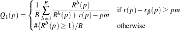
The resampling methodology for the BOOTSTRAP and PERMUTATION methods is used to create B resamples. For the bth resample, let $R^ b(p)$ denote the number of p-values that are less than or equal to the observed p-value p. Let $r_\beta (p)$ be the 100 $(1-\beta )$ quantile of $\{ R^1(p)\ldots R^ b(p)\ldots R^ B(p)\}$ , and let $r(p)$ be the number of observed p-values less than or equal to p. Compute one of the following estimators:

local estimator	$\displaystyle Q_1(p)=\begin{cases} \displaystyle \nonumber \frac{1}{B}\sum _{b=1}^{B} \frac{R^ b(p)}{R^ b(p)+r(p)-pm} & \mbox{if } r(p)-r_\beta (p) \ge pm \\ \displaystyle \# \{ R^ b(p)\ge 1\} /B & \mbox{otherwise}\end{cases}$
upper limit estimator	$\displaystyle Q_\beta (p)=\begin{cases} \displaystyle \nonumber \sup _{x\in [0,p]} \left( \frac{1}{B}\sum _{b=1}^{B} \frac{R^ b(x)}{R^ b(x)+r(x)-r_\beta (x)}\right) & \mbox{if } r(x)-r_\beta (x) \ge 0 \\ \displaystyle \# \{ R^ b(p)\ge 1\} /B & \mbox{otherwise}\end{cases}$

where m is the number of tests and B is the number of resamples. Then for $Q=Q_1$ or $Q_\beta$ , the adjusted p-values are computed as

$\begin{equation*} \tilde{p}_{(i)} = \begin{cases} Q(p_{(m)}) & \mbox{for } i=m \\ \min \left( \tilde{p}_{(i+1)} , Q(p_{(i)}) \right) & \mbox{for } i=m-1,\ldots ,1 \end{cases}\end{equation*}$

Adaptive False Discovery Rate

Since the FDR method controls the false discovery rate at $\le \frac{m_0}{m}\alpha \le \alpha$ , knowledge of $m_0$ allows improvement of the power of the adjustment while still maintaining control of the false discovery rate. The ADAPTIVEFDR option requests adaptive adjusted p-values for approximate control of the false discovery rate, as discussed in Benjamini and Hochberg (2000). See the section Adaptive Adjustments for more details. These adaptive adjustments are also defined in step-up fashion but use an estimate $\hat{m}_0$ of the number of true null hypotheses:

$\begin{equation*} \tilde{p}_{(i)} = \begin{cases} \frac{\hat{m}_0}{m}p_{(m)} & \mbox{for } i=m \\ \min \left( \tilde{p}_{(i+1)} , \frac{\hat{m}_0}{i} p_{(i)} \right) & \mbox{for } i=m-1,\ldots ,1 \end{cases}\end{equation*}$

Since $\hat{m}_0 \le m$ , the larger p-values are adjusted down. This means that, as defined, controlling the false discovery rate enables you to reject these tests at a level less than the observed p-value. However, by default, this reduction is prevented with an additional restriction: $\tilde{p}_{(i)}=\max \{ \tilde{p}_{(i)},p_{(i)}\}$ .

To use this adjustment, Benjamini and Hochberg (2000) suggest first specifying the FDR option—if at least one test is rejected at your level, then apply the ADAPTIVEFDR adjustment. Alternatively, Benjamini, Krieger, and Yekutieli (2006) apply the FDR adjustment at level $\frac{\alpha }{\alpha +1}$ , then specify the resulting number of true hypotheses with the NTRUENULL= option and apply the ADAPTIVEFDR adjustment; they show that this two-stage linear step-up procedure controls the false discovery rate at level $\alpha$ for independent test statistics.

Positive False Discovery Rate

The PFDR option computes the “q-values” $\hat{q}_{\lambda }(p_ i)$ (Storey, 2002; Storey, Taylor, and Siegmund, 2004), which are adaptive adjusted p-values for strong control of the false discovery rate when the p-values corresponding to the true null hypotheses are independent and uniformly distributed. There are four versions of the PFDR available. Let $N(\lambda )$ be the number of observed p-values that are less than or equal to $\lambda$ ; let m be the number of tests; let f = 1 if the FINITE option is specified, and otherwise set f = 0; and denote the estimated proportion of true null hypotheses by

$\hat{\pi }_0(\lambda ) = \frac{m-N(\lambda )+f}{(1-\lambda )m}$

The default estimate of FDR is

$\widehat{\hbox{FDR}}_{\lambda }(p) = \frac{\hat{\pi }_0(\lambda ) p}{\max (N(p), 1)/m}$

If you set $\lambda =0$ , then this is identical to the FDR adjustment.

The positive FDR is estimated by

$\widehat{\hbox{pFDR}}_{\lambda }(p) = \frac{ \widehat{\hbox{FDR}}_{\lambda }(p)}{1-(1-p)^ m}$

The finite-sample versions of these two estimators for independent null p-values are given by

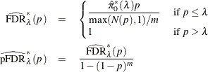
$\begin{eqnarray*} \widehat{\hbox{FDR}}_{\lambda }^{*}(p) & =& \begin{cases} \displaystyle \nonumber \frac{\hat{\pi }_0^{*}(\lambda ) p}{\max (N(p),1)/m} & \mbox{ if } p\le \lambda \\ \displaystyle 1 & \mbox{ if } p > \lambda \end{cases}\\ \widehat{\hbox{pFDR}}_{\lambda }^{*}(p) & =& \frac{ \widehat{\hbox{FDR}}_{\lambda }^{*}(p)}{1-(1-p)^ m} \\ \end{eqnarray*}$

Finally, the adjusted p-values are computed as

$\tilde{p}_ i= \hat{q}_{\lambda }(p_ i) = \inf _{p\ge p_ i}{\hbox{FDR}}_{\lambda }(p) \quad i=1,\ldots ,m$

This method can produce adjusted p-values that are smaller than the raw p-values. This means that, as defined, controlling the false discovery rate enables you to reject these tests at a level less than the observed p-value. However, by default, this reduction is prevented with an additional restriction: $\tilde{p}_{i}=\max \{ \tilde{p}_{i},p_{i}\}$ .

The MULTTEST Procedure