The MI Procedure

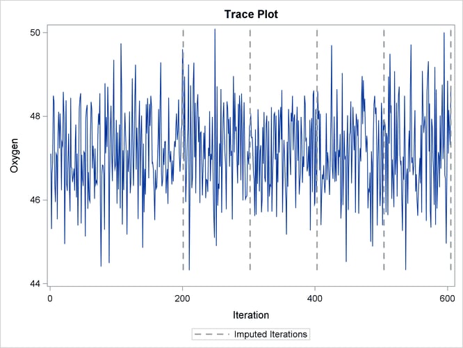
This example uses the MCMC method with a single chain. It also displays trace and autocorrelation plots to check convergence for the single chain.

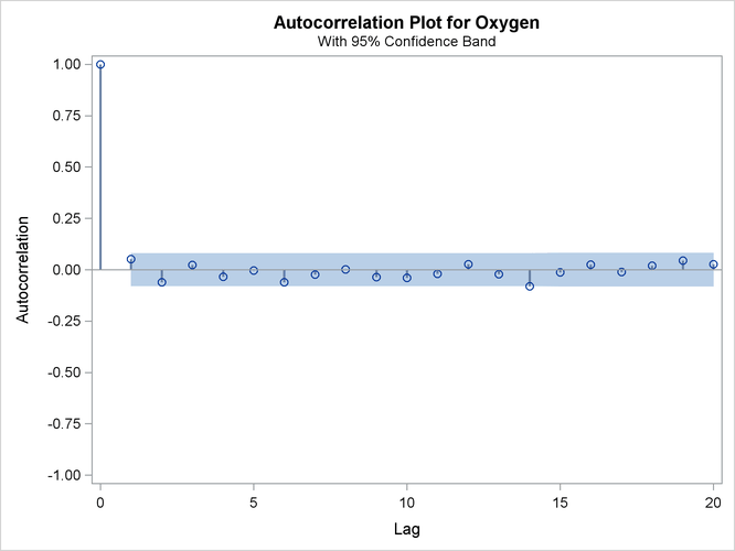
The following statements use the MCMC method to create an iteration plot for the successive estimates of the mean of Oxygen. These statements also create an autocorrelation function plot for the variable Oxygen.

ods graphics on;
proc mi data=Fitness1 seed=501213 mu0=50 10 180;
   mcmc plots=(trace(mean(Oxygen)) acf(mean(Oxygen)));
   var Oxygen RunTime RunPulse;
run;
ods graphics off;

With ODS Graphics enabled, the TRACE(MEAN(OXYGEN)) option in the PLOTS= option displays the trace plot of means for the variable Oxygen, as shown in Output 61.11.1. The dashed vertical lines indicate the imputed iterations—that is, the Oxygen values used in the imputations. The plot shows no apparent trends for the variable Oxygen.

The ACF(MEAN(OXYGEN)) option in the PLOTS= option displays the autocorrelation plot of means for the variable Oxygen, as shown in Output 61.11.2. The autocorrelation function plot shows no significant positive or negative autocorrelation.

You can also create plots for the worst linear function, the means of other variables, the variances of variables, and the covariances between variables. Alternatively, you can use the OUTITER option to save statistics such as the means, standard deviations, covariances, –2 log LR statistic, –2 log LR statistic of the posterior mode, and worst linear function from each iteration in an output data set. Then you can do a more in-depth trace (time series) analysis of the iterations with other procedures, such as PROC AUTOREG and PROC ARIMA in the SAS/ETS User's Guide.

For general information about ODS Graphics, see Chapter 21: Statistical Graphics Using ODS. For specific information about the graphics available in the MI procedure, see the section ODS Graphics.