The LOESS Procedure
-
Overview

-
Getting Started
-
Syntax
-
DetailsMissing ValuesOutput Data SetsData ScalingDirect versus Interpolated Fittingk-d Trees and BlendingLocal WeightingIterative ReweightingSpecifying the Local PolynomialsSmoothing MatrixModel Degrees of FreedomStatistical Inference and Lookup Degrees of FreedomAutomatic Smoothing Parameter SelectionSparse and Approximate Degrees of Freedom ComputationScoring Data SetsODS Table NamesODS Graphics
-
Examples
- References
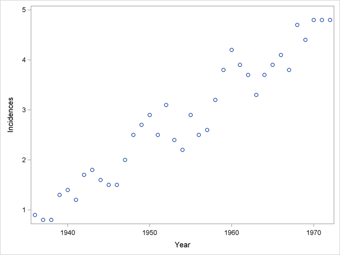
The following data from the Connecticut Tumor Registry presents age-adjusted numbers of melanoma incidences per 100,000 people for the 37 years from 1936 to 1972 (Houghton, Flannery, and Viola, 1980).
data Melanoma;
   input  Year Incidences @@;
   format Year d4.0;
   datalines;
1936    0.9   1937   0.8  1938   0.8  1939   1.3
1940    1.4   1941   1.2  1942   1.7  1943   1.8
1944    1.6   1945   1.5  1946   1.5  1947   2.0
1948    2.5   1949   2.7  1950   2.9  1951   2.5
1952    3.1   1953   2.4  1954   2.2  1955   2.9
1956    2.5   1957   2.6  1958   3.2  1959   3.8
1960    4.2   1961   3.9  1962   3.7  1963   3.3
1964    3.7   1965   3.9  1966   4.1  1967   3.8
1968    4.7   1969   4.4  1970   4.8  1971   4.8
1972    4.8
;
The following PROC SGPLOT statements produce the simple scatter plot of these data displayed in Figure 57.1.
proc sgplot data=Melanoma;
   scatter y=Incidences x=Year;
run;
Suppose that you want to smooth the response variable Incidences as a function of the variable Year. The following PROC LOESS statements request this analysis with the default settings:
ods graphics on;

proc loess data=Melanoma;
   model Incidences=Year;
run;
You use the PROC LOESS statement to invoke the procedure and specify the data set. The MODEL statement names the dependent and independent variables.
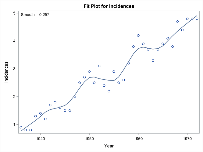
When ODS Graphics is enabled, PROC LOESS produces several default plots. Figure 57.2 shows the “Fit Plot” that overlays the loess fit on a scatter plot of the data. You can see that the loess fit captures the increasing trend in the data as well as the periodic pattern in the data, which is related to an 11-year sunspot activity cycle.
Figure 57.3: Fit Summary
| Fit Summary | |
|---|---|
| Fit Method | kd Tree |
| Blending | Linear |
| Number of Observations | 37 |
| Number of Fitting Points | 37 |
| kd Tree Bucket Size | 1 |
| Degree of Local Polynomials | 1 |
| Smoothing Parameter | 0.25676 |
| Points in Local Neighborhood | 9 |
| Residual Sum of Squares | 2.03105 |
| Trace[L] | 8.62243 |
| GCV | 0.00252 |
| AICC | -1.17277 |
Figure 57.3 shows the “Fit Summary” table. This table details the settings used and provides statistics about the fit that is produced. You can see that smoothing parameter value for this loess fit is 0.257. This smoothing parameter determines the fraction of the data in each local neighborhood. In this example, there are 37 data points and so the smoothing parameter value of 0.257 yields local neighborhoods containing 9 observations.
Figure 57.4: Smoothing Parameter Selection
| Optimal Smoothing Criterion | |
|---|---|
| AICC | Smoothing Parameter |
| -1.17277 | 0.25676 |
The “Smoothing Criterion” table provides information about how this smoothing parameter value is selected. The default method implemented in PROC LOESS chooses the smoothing parameter that minimizes the AICC criterion (Hurvich, Simonoff, and Tsai, 1998) that strikes a balance between the residual sum of squares and the complexity of the fit.
You use options in the MODEL statement to change the default settings and request optionally displayed tables. For example, the following statements request that the “Model Summary” and “Output Statistics” tables be included in the displayed output. By default, these tables are not displayed.
proc loess data=Melanoma;
   model Incidences=Year / details(ModelSummary OutputStatistics);
run;
Figure 57.5: Model Summary Table
| Model Summary | ||||
|---|---|---|---|---|
| Smoothing Parameter |
Local Points |
Residual SS | GCV | AICC |
| 0.41892 | 15 | 3.42229 | 0.00339 | -0.96252 |
| 0.68919 | 25 | 4.05838 | 0.00359 | -0.93459 |
| 0.31081 | 11 | 2.51054 | 0.00279 | -1.12034 |
| 0.20270 | 7 | 1.58513 | 0.00239 | -1.12221 |
| 0.17568 | 6 | 1.56896 | 0.00241 | -1.09706 |
| 0.28378 | 10 | 2.50487 | 0.00282 | -1.10402 |
| 0.20270 | 7 | 1.58513 | 0.00239 | -1.12221 |
| 0.25676 | 9 | 2.03105 | 0.00252 | -1.17277 |
| 0.22973 | 8 | 2.02965 | 0.00256 | -1.15145 |
| 0.25676 | 9 | 2.03105 | 0.00252 | -1.17277 |
The “Model Summary” table shown in Figure 57.5 provides information about all the models that PROC LOESS evaluated in choosing the smoothing parameter value.
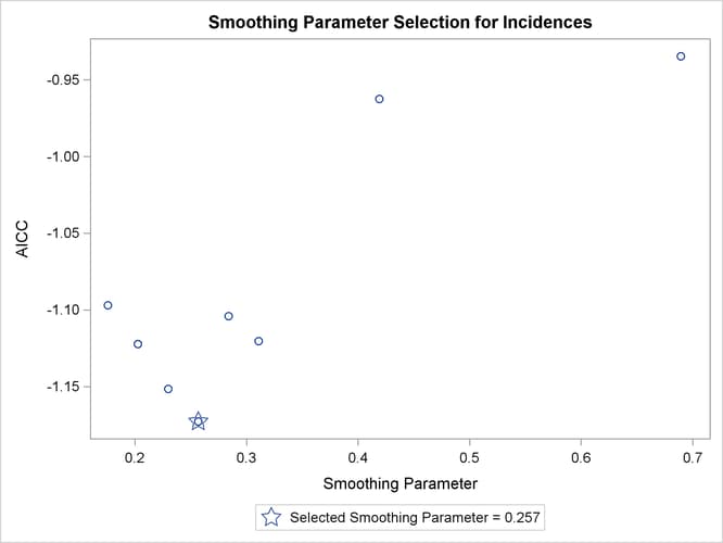
Figure 57.6 shows the “Criterion Plot” that provides a graphical display of the smoothing parameter selection process.
Figure 57.7: Output Statistics
| Output Statistics | ||||
|---|---|---|---|---|
| Obs | Year | Incidences | Predicted Incidences | Residual |
| 1 | 1936 | 0.90000 | 0.76235 | 0.13765 |
| 2 | 1937 | 0.80000 | 0.88992 | -0.08992 |
| 3 | 1938 | 0.80000 | 1.01764 | -0.21764 |
| 4 | 1939 | 1.30000 | 1.14303 | 0.15697 |
| 5 | 1940 | 1.40000 | 1.28654 | 0.11346 |
| 6 | 1941 | 1.20000 | 1.44528 | -0.24528 |
| 7 | 1942 | 1.70000 | 1.53482 | 0.16518 |
| 8 | 1943 | 1.80000 | 1.57895 | 0.22105 |
| 9 | 1944 | 1.60000 | 1.62058 | -0.02058 |
| 10 | 1945 | 1.50000 | 1.68627 | -0.18627 |
| 11 | 1946 | 1.50000 | 1.82449 | -0.32449 |
| 12 | 1947 | 2.00000 | 2.04976 | -0.04976 |
| 13 | 1948 | 2.50000 | 2.30981 | 0.19019 |
| 14 | 1949 | 2.70000 | 2.53653 | 0.16347 |
| 15 | 1950 | 2.90000 | 2.68921 | 0.21079 |
| 16 | 1951 | 2.50000 | 2.70779 | -0.20779 |
| 17 | 1952 | 3.10000 | 2.64837 | 0.45163 |
| 18 | 1953 | 2.40000 | 2.61468 | -0.21468 |
| 19 | 1954 | 2.20000 | 2.58792 | -0.38792 |
| 20 | 1955 | 2.90000 | 2.57877 | 0.32123 |
| 21 | 1956 | 2.50000 | 2.71078 | -0.21078 |
| 22 | 1957 | 2.60000 | 2.96981 | -0.36981 |
| 23 | 1958 | 3.20000 | 3.26005 | -0.06005 |
| 24 | 1959 | 3.80000 | 3.54143 | 0.25857 |
| 25 | 1960 | 4.20000 | 3.73482 | 0.46518 |
| 26 | 1961 | 3.90000 | 3.78186 | 0.11814 |
| 27 | 1962 | 3.70000 | 3.74362 | -0.04362 |
| 28 | 1963 | 3.30000 | 3.70904 | -0.40904 |
| 29 | 1964 | 3.70000 | 3.72917 | -0.02917 |
| 30 | 1965 | 3.90000 | 3.82382 | 0.07618 |
| 31 | 1966 | 4.10000 | 4.00515 | 0.09485 |
| 32 | 1967 | 3.80000 | 4.18573 | -0.38573 |
| 33 | 1968 | 4.70000 | 4.35152 | 0.34848 |
| 34 | 1969 | 4.40000 | 4.50284 | -0.10284 |
| 35 | 1970 | 4.80000 | 4.64413 | 0.15587 |
| 36 | 1971 | 4.80000 | 4.78291 | 0.01709 |
| 37 | 1972 | 4.80000 | 4.91602 | -0.11602 |
Figure 57.7 show the “Output Statistics” table that contains the predicted loess fit value at each observation in the input data set.
Although the default method for selecting the smoothing parameter value is often satisfactory, it is often a good practice to examine how the loess fit varies with the smoothing parameter. In some cases, fits with different smoothing parameters might reveal important features of the data that cannot be discerned by looking at a fit with just a single “best” smoothing parameter. Example 57.4 provides such an example. You can produce the loess fits for a range of smoothing parameters by using the SMOOTH= option in the MODEL statement as follows:
proc loess data=Melanoma;
   model Incidences=Year/smooth=0.1 0.25 0.4 0.6 residual;
   ods output OutputStatistics=Results;
run;
The RESIDUAL option causes the residuals to be added to the “Output Statistics” table. Note that, even if you do not specify the DETAILS option in the MODEL statement to request the display of the “Output Statistics” table, you can use an ODS OUTPUT statement to output this and other optionally displayed tables as data sets.
PROC PRINT displays the first five observations of the Results data set:
proc print data=Results(obs=5);
   id obs;
run;
Figure 57.8: PROC PRINT Output of the Results Data Set
| Obs | SmoothingParameter | Year | DepVar | Pred | Residual |
|---|---|---|---|---|---|
| 1 | 0.1 | 1936 | 0.9 | 0.90000 | 0 |
| 2 | 0.1 | 1937 | 0.8 | 0.80000 | 0 |
| 3 | 0.1 | 1938 | 0.8 | 0.80000 | 0 |
| 4 | 0.1 | 1939 | 1.3 | 1.30000 | 0 |
| 5 | 0.1 | 1940 | 1.4 | 1.40000 | 0 |
Note that the fits for all the smoothing parameters are placed in single data set. A variable named SmoothingParameter that you use to distinguish each fit is included in this data set.
When you specify a list of smoothing parameters for a model and ODS Graphics is enabled, PROC LOESS produces a panel containing up to six plots that show the fit obtained for each value of the smoothing parameter that you specify. If you specify more than six smoothing values, then multiple panels are produced. For each regressor, PROC LOESS also produces panels of the residuals versus each regressor by the smoothing parameters that you specify.
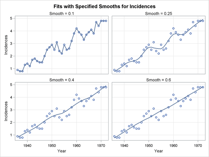
If you examine the plots in Figure 57.9, you see that a visually reasonable fit is obtained with smoothing parameter values of 0.25. With smoothing parameter value 0.1, there is gross overfitting in the sense that the original data are exactly interpolated. When the smoothing parameter value is 0.4, you obtain an overly smooth fit where the contribution of the sunspot cycle has been mostly averaged away. At smoothing parameter value 0.6 the fit shows just the increasing trend in the data.
It is also instructive to look at scatter plots of the residuals for each of the fits. These are also produced by default by PROC LOESS when ODS Graphics is enabled.
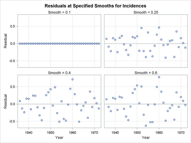
Figure 57.10 shows a scatter plot of the residuals by year for each smoothing parameter value. One way to discern patterns in these residuals
is to superimpose a loess fit on each plot in the panel. You request loess fits on the residual plots in this panel by specifying
the SMOOTH= suboption of the PLOTS=RESIDUALSBYSMOOTH option in the PROC LOESS statement. Note that the loess fits that are displayed on each of the residual plots are obtained independently of the loess
fit that produces these residuals. The following statements show how you do this for the Melanoma data.
proc loess data=Melanoma plots=ResidualsBySmooth(smooth);
   model Incidences=Year/smooth=0.1 0.25 0.4 0.6;
run;
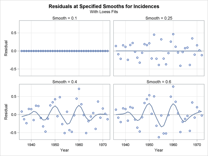
The loess fits shown on the plots in Figure 57.11 help confirm the conclusions obtained when you look at Figure 57.9. Note that residuals for smoothing parameter value 0.25 do not exhibit any pattern, confirming that at this value the loess fit of the melanoma data has successfully modeled the variation in this data. By contrast, the residuals for the fit with smoothing parameter 0.6 retain the variation caused by the sunspot cycle.
The examination of the fits and residuals obtained with a range of smoothing parameter values confirms that the value of 0.257 that PROC LOESS selects automatically is appropriate for these data. The next step in this analysis is to examine fit diagnostics and produce confidence limit for the fit. If ODS Graphics is enabled, then a panel of fit diagnostics is produced. Furthermore, you can request prediction confidence limits by adding the CLM option in the MODEL statement. By default 95% limits are produced, but you can use the ALPHA= option in the MODEL statement to change the significance level. The following statements request 90% confidence limits.
proc loess data=Melanoma;
   model Incidences=Year/clm alpha=0.1;
run;

ods graphics off;
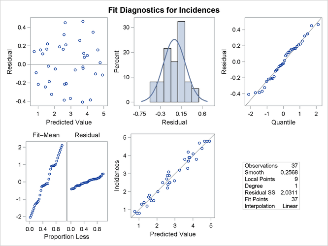
Figure 57.12 shows the fit diagnostics panel. The histogram of the residuals with overlaid normal density estimator and the normal quantile plot show that the residuals do exhibit some small departure from normality. The “Residual-Fit” spread plot shows that the spread in the centered fit is much wider that the spread in the residuals. This indicates that the fit has accounted for most of the variation in the incidences of melanoma in this data. This conclusion is supported by the absence of any clear pattern in the scatter plot of residuals by predicted values and the closeness of the points to the 45-degree reference line in the plot of observed by predicted values.

Finally, Figure 57.13 shows the selected loess fit with 90% confidence limits.