The LOESS Procedure
-
Overview

-
Getting Started
-
Syntax
-
DetailsMissing ValuesOutput Data SetsData ScalingDirect versus Interpolated Fittingk-d Trees and BlendingLocal WeightingIterative ReweightingSpecifying the Local PolynomialsSmoothing MatrixModel Degrees of FreedomStatistical Inference and Lookup Degrees of FreedomAutomatic Smoothing Parameter SelectionSparse and Approximate Degrees of Freedom ComputationScoring Data SetsODS Table NamesODS Graphics
-
Examples
- References
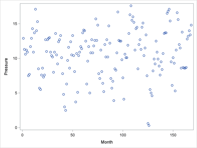
The data set sashelp.ENSO, which is available in the Sashelp library, contains measurements of monthly averaged atmospheric pressure differences between Easter Island and Darwin, Australia,
for a period of 168 months (National Institute of Standards and Technology, 1998).
The following PROC SGPLOT statements produce the simple scatter plot of the ENSO data, displayed in Output 57.4.1.
proc sgplot data=sashelp.ENSO;
   scatter y=Pressure x=Month;
run;
You can compute a loess fit and obtain graphical results for these data by using the following statements:
ods graphics on;

proc loess data=sashelp.ENSO plots=residuals(smooth);
   model Pressure=Month;
run;
The “Smoothing Criterion” and “Fit Summary” tables are shown in Output 57.4.2, and the fit plot is shown in Output 57.4.3.
Output 57.4.2: Output from PROC LOESS
| Optimal Smoothing Criterion | |
|---|---|
| AICC | Smoothing Parameter |
| 3.41105 | 0.22321 |
| Fit Summary | |
|---|---|
| Fit Method | kd Tree |
| Blending | Linear |
| Number of Observations | 168 |
| Number of Fitting Points | 33 |
| kd Tree Bucket Size | 7 |
| Degree of Local Polynomials | 1 |
| Smoothing Parameter | 0.22321 |
| Points in Local Neighborhood | 37 |
| Residual Sum of Squares | 1654.27725 |
| Trace[L] | 8.74180 |
| GCV | 0.06522 |
| AICC | 3.41105 |
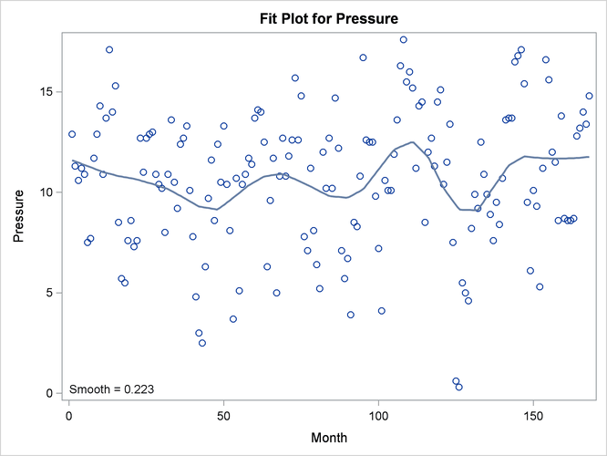
This weather-related data should exhibit an annual cycle. However, the loess fit in Output 57.4.3 indicates a longer cycle but no annual cycle. This suggests that the loess fit is oversmoothed. One way to detect oversmoothing is to look for patterns in the fit residuals. With ODS Graphics enabled, PROC LOESS produces a scatter plot of the residuals versus each regressor in the model. To aid in visually detecting patterns in these scatter plots, it is useful to superimpose a nonparametric fit on these scatter plots. You can request this by specifying the SMOOTH suboption of the PLOTS=RESIDUALS option in the PROC LOESS statement. The nonparametric fit that is produced is again a loess fit that is produced independently of the loess fit used to obtain these residuals.
With the superimposed loess fit shown in Output 57.4.4, you can clearly identify an annual cycle in the residuals, which confirms that the loess fit for the ENSO is oversmoothed. What accounts for this poor fit?

The smoothing parameter value used for the loess fit shown in Output 57.4.3 was chosen using the default method of PROC LOESS, namely a golden section minimization of the AICC criterion over the interval
![]() . One possibility is that the golden section search has found a local rather than a global minimum of the AICC criterion.
You can test this by redoing the fit requesting a global minimum. You do this with the following statements:
. One possibility is that the golden section search has found a local rather than a global minimum of the AICC criterion.
You can test this by redoing the fit requesting a global minimum. You do this with the following statements:
proc loess data=sashelp.ENSO;
   model Pressure=Month/select=AICC(global);
run;
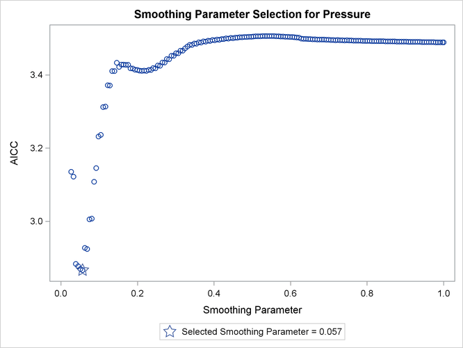
The explanation for the oversmoothed fit in Output 57.4.3 is now apparent. Output 57.4.5 shows that the golden section search algorithm found the local minimum that occurs near the value 0.22 of the smoothing parameter rather than the global minimum that occurs near 0.06. Note that if you restrict the range of smoothing parameter values examined to lie below 0.2, then the golden section search finds the global minimum, as the following statements demonstrate:
proc loess data=sashelp.ENSO;
   model Pressure=Month/select=AICC(range(0.03,0.2));
run;
Output 57.4.6: Selected Smoothing Parameter Value
| Optimal Smoothing Criterion | |
|---|---|
| AICC | Smoothing Parameter |
| 2.86660 | 0.05655 |
Output 57.4.6 shows that with the restricted range of smoothing parameter values examined, PROC LOESS finds the global minimum of the AICC criterion. Often you might not know an appropriate range of smoothing parameter values to examine. In such cases, you can use the PRESEARCH suboption of the SELECT= option in the MODEL statement. When you specify this option, PROC LOESS does a preliminary search to try to locate a smoothing parameter value range that contains just the first local minimum of the criterion being used for the selection. The following statements provide an example.
proc loess data=sashelp.ENSO plots=residuals(smooth);
   model Pressure=Month/select=AICC(presearch);
run;

ods graphics off;
Output 57.4.7: Selected Smoothing Parameter Value When Presearch Is Specified
| Optimal Smoothing Criterion | |
|---|---|
| AICC | Smoothing Parameter |
| 2.86660 | 0.05655 |
Output 57.4.7 shows that with the PRESEARCH suboption specified, PROC LOESS selects the smoothing parameter value that yields the global minimum of the AICC criterion. The fit obtained is shown in Output 57.4.8, and a plot of the residuals with a superimposed loess fit is shown in Output 57.4.9.


In contrast to the residual plot show in Output 57.4.4, the residuals plotted in Output 57.4.9 do not exhibit any pattern, indicating that the corresponding loess fit has captured all the systematic variation in the data.
An interesting question is whether there is some phenomenon captured in the data that would explain the presence of the local minimum near 0.22 in the AICC curve. Note that there is some evidence of a cycle of about 42 months in the oversmoothed fit in Output 57.4.3. You can see this cycle because the strong annual cycle in Output 57.4.8 has been smoothed out. The physical phenomenon that accounts for the existence of this cycle has been identified as the periodic warming of the Pacific Ocean known as “El Niño.”