The NLIN Procedure

Example 63.7 Parameter Profiling

The following model, taken from Clarke (1987), demonstrates the benefits of parameter profiling and confidence curves to identify the nonlinear characteristics of parameters that occur in the model. The profiling is also augmented with a plot that shows the influence of each observation on the parameter estimates.

The model takes the form

$\mr {E}[Y|x] = \theta _3 + \theta _2 \exp \{ \theta _1 x \}$

The data set used in this example is taken from Clarke (1987). The following DATA step creates this data set:

data clarke1987a;
   input  x y;
   datalines;
1    3.183
2    3.059
3    2.871
4    2.622
5    2.541
6    2.184
7    2.110
8    2.075
9    2.018
10   1.903
11   1.770
12   1.762
13   1.550
;

The model is fit with the following statements in the NLIN procedure:

ods graphics on;
proc nlin data=clarke1987a plots(stats=none)=diagnostics;
   parms theta1=-0.15
         theta2=2.0 
         theta3=0.80; 
   profile theta3 / range = -6 to 2 by 0.2 all;  
   model y = theta3 + theta2*exp(theta1*x);   
run;
ods graphics off;

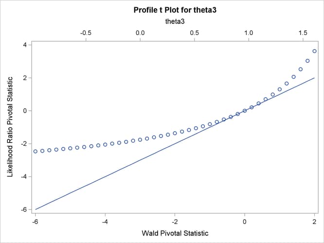
The profile t plot, Output 63.7.1, for parameter $\theta _3$ shows a definite deviation from the linear reference line that has a slope of 1 and passes through the origin. Hence, Wald-based inference for $\theta _3$ is not appropriate. The confidence curve for $\theta _3$ validates this conclusion.

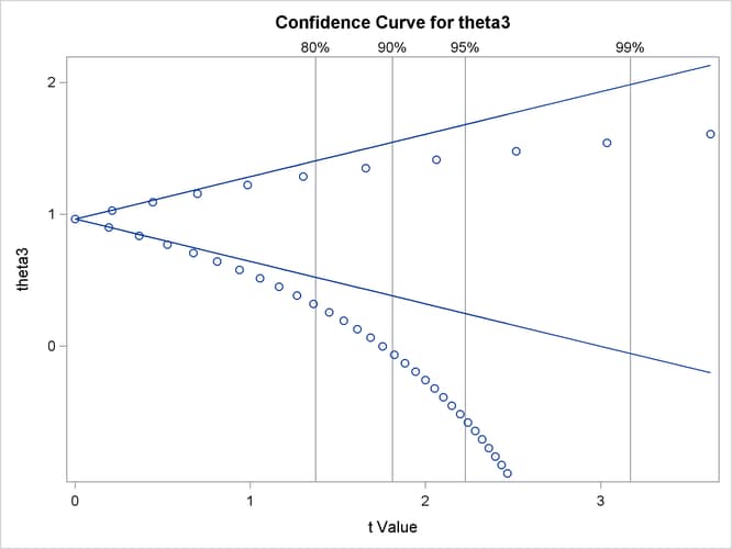
Output 63.7.2 shows the confidence curve for $\theta _3$ . You can see that there is a significant difference between the Wald-based confidence interval and the corresponding likelihood-based interval. In such cases, the likelihood-based intervals are preferred because their coverage rate is much closer to the nominal values than the coverage rate of the Wald-based intervals (Donaldson and Schnabel, 1987; Cook and Weisberg, 1990). Furthermore, this example shows that the adequacy of a linear approximation with regards to a certain parameter cannot be inferred directly from the model. If it could, $\theta _3$ , which enters the model linearly, would have a completely linear behavior. For a detailed discussion about this issue, see Cook and Weisberg (1990).

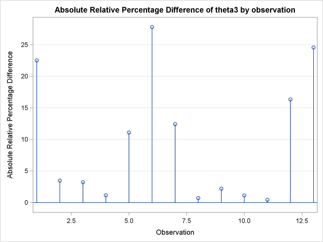
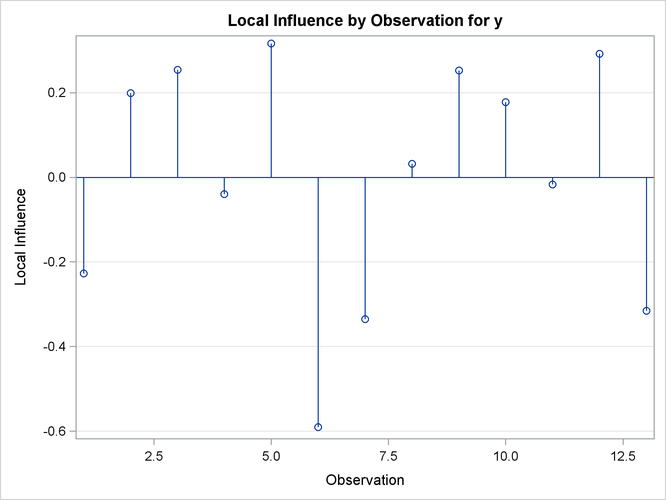
Finally, Output 63.7.3 depicts the influence of each observation on the value of $\theta _3$ . Observations 6 and 13 have the most influence on the value of this parameter. The plot is generated using the leave-one-out method and should be contrasted with the local influence plot, Output 63.7.4, which is based on assessing the influence of an additive perturbation of the response variable.

Output 63.7.1: Profile t Plot

Output 63.7.2: Confidence Curve

Output 63.7.3: Observation Influence on Parameter Estimate

Output 63.7.4: Local Influence Plot