The NLIN Procedure
- Overview
-
Getting Started

-
Syntax
-
DetailsAutomatic DerivativesMeasures of Nonlinearity and DiagnosticsMissing ValuesSpecial VariablesTroubleshootingComputational MethodsOutput Data SetsConfidence IntervalsCovariance Matrix of Parameter EstimatesConvergence MeasuresDisplayed OutputIncompatibilities with SAS 6.11 and Earlier Versions of PROC NLINODS Table NamesODS Graphics
-
Examples
- References
The model in this example, taken from St. Laurent and Cook (1993), shows an unusual behavior in that the intrinsic curvature is substantially larger than the parameter-effects curvature. This example demonstrates how the diagnostics features of PROC NLIN can be used to perform postconvergence diagnostics.
The model takes the form
The following DATA step creates a small data set to be used in this example:
data contrived;
   input x1 x2 y;
   datalines;
-4.0   -2.5  -10.0
-3.0   -2.0   -5.0
-2.0   -1.5   -2.0
-1.0   -1.0   -1.0
 0.0    0.0    1.5
 1.0    1.0    4.0
 2.0    1.5    5.0
 3.0    2.0    6.0
 4.0    2.5    7.0
-3.5   -2.2   -7.1
-3.5   -1.7   -5.1
 3.5    0.7    6.1
 2.5    1.2    7.5
;
The model is fit with the following statements in the NLIN procedure:
ods graphics on;
proc nlin data=contrived bias hougaard
        NLINMEASURES plots(stats=all)=(diagnostics);
   parms alpha=2.0
         gamma=0.0;
   model y = alpha*x1 + exp(gamma*x2);
run;
ods graphics off;
Output 63.6.1: Bias, Skewness, and Global Nonlinearity Measures
| Parameter | Estimate | Approx Std Error |
Approximate 95% Confidence Limits |
Skewness | Bias | Percent Bias |
|
|---|---|---|---|---|---|---|---|
| alpha | 1.9378 | 0.4704 | 0.9024 | 2.9733 | 6.6491 | 0.5763 | 29.7 |
| gamma | 0.0718 | 0.7923 | -1.6720 | 1.8156 | -7.5596 | -0.9982 | -1390 |
| Global Nonlinearity Measures | |
|---|---|
| Max Intrinsic Curvature | 6.6007 |
| RMS Intrinsic Curvature | 4.0421 |
| Max Parameter-Effects Curvature | 3.5719 |
| RMS Parameter-Effects Curvature | 2.1873 |
| Curvature Critical Value | 0.5011 |
| Raw Residual Variance | 2.1722 |
| Projected Residual Variance | 1.4551 |
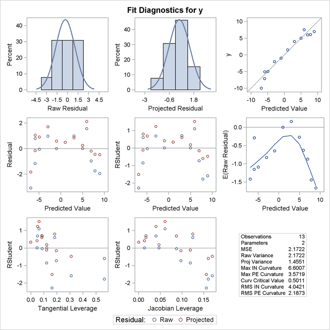
The bias, skewness, and both the maximum and RMS intrinsic curvatures, compared to the critical curvature value, show that the model is highly nonlinear (Output 63.6.1). As such, performing diagnostics with the raw residuals can be problematic because they might have undesirable statistical properties: a nonzero mean and a negative semidefinite (instead of zero) covariance with the predicted values and different variances. In addition, the use of tangential leverage is questionable in this case.
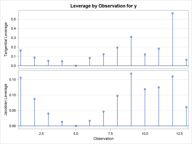
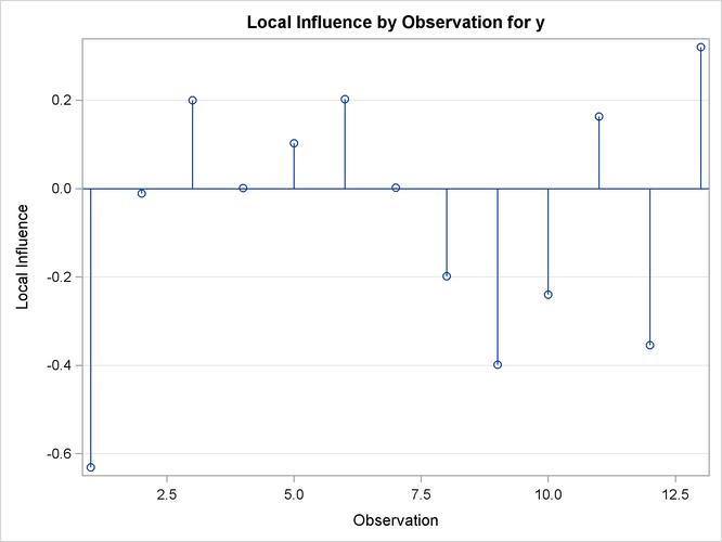
The partial results from this NLIN run are shown in Output 63.6.2, Output 63.6.3, and Output 63.6.4. The diagnostics plots corroborate the previously mentioned expectations: highly correlated raw residuals (with the predicted values), significant differences between tangential and Jacobian leverages and projected residuals which overcome some of the shortcomings of the raw residuals. Finally, considering the large intrinsic curvature, reparameterization might not make the model close-to-linear, perhaps necessitating the construction of another model.