The MCMC Procedure
-
Overview

-
Getting Started
-
Syntax
-
DetailsHow PROC MCMC WorksBlocking of ParametersSampling MethodsTuning the Proposal DistributionDirect SamplingConjugate SamplingInitial Values of the Markov ChainsAssignments of ParametersStandard DistributionsUsage of Multivariate DistributionsSpecifying a New DistributionUsing Density Functions in the Programming StatementsTruncation and CensoringSome Useful SAS FunctionsMatrix Functions in PROC MCMCCreate Design MatrixModeling Joint LikelihoodRegenerating Diagnostics PlotsCaterpillar PlotAutocall Macros for PostprocessingGamma and Inverse-Gamma DistributionsPosterior Predictive DistributionHandling of Missing DataFunctions of Random-Effects ParametersFloating Point Errors and OverflowsHandling Error MessagesComputational ResourcesDisplayed OutputODS Table NamesODS Graphics
-
ExamplesSimulating Samples From a Known DensityBox-Cox TransformationLogistic Regression Model with a Diffuse PriorLogistic Regression Model with Jeffreys’ PriorPoisson RegressionNonlinear Poisson Regression ModelsLogistic Regression Random-Effects ModelNonlinear Poisson Regression Multilevel Random-Effects ModelMultivariate Normal Random-Effects ModelMissing at Random AnalysisNonignorably Missing Data (MNAR) AnalysisChange Point ModelsExponential and Weibull Survival AnalysisTime Independent Cox ModelTime Dependent Cox ModelPiecewise Exponential Frailty ModelNormal Regression with Interval CensoringConstrained AnalysisImplement a New Sampling AlgorithmUsing a Transformation to Improve MixingGelman-Rubin Diagnostics
- References
This example illustrates how to fit a logistic regression model with a diffuse prior in PROC MCMC. You can also use the BAYES statement in PROC GENMOD. See Chapter 40: The GENMOD Procedure.
The following statements create a SAS data set with measurements of the number of deaths, y, among n beetles that have been exposed to an environmental contaminant x:
title 'Logistic Regression Model with a Diffuse Prior';
data beetles;
   input n y x @@;
   datalines;
6  0  25.7   8  2  35.9   5  2  32.9   7  7  50.4   6  0  28.3
7  2  32.3   5  1  33.2   8  3  40.9   6  0  36.5   6  1  36.5
6  6  49.6   6  3  39.8   6  4  43.6   6  1  34.1   7  1  37.4
8  2  35.2   6  6  51.3   5  3  42.5   7  0  31.3   3  2  40.6
;
You can model the data points ![]() with a binomial distribution,
with a binomial distribution,
where ![]() is the success probability and links to the regression covariate
is the success probability and links to the regression covariate ![]() through a logit transformation:
through a logit transformation:
The priors on ![]() and
and ![]() are both diffuse normal:
are both diffuse normal:
|
|
|
|
|
|
|
|
These statements fit a logistic regression with PROC MCMC:
ods graphics on;
proc mcmc data=beetles ntu=1000 nmc=20000 nthin=2 propcov=quanew
          diag=(mcse ess) outpost=beetleout seed=246810;
   ods select PostSummaries PostIntervals mcse ess TADpanel;
   parms (alpha  beta) 0;
   prior alpha beta ~ normal(0, var = 10000);
   p = logistic(alpha + beta*x);
   model y ~ binomial(n,p);
run;
The key statement in the program is the assignment to p that calculates the probability of death. The SAS function LOGISTIC does the proper transformation. The MODEL statement specifies that the response variable, y, is binomially distributed with parameters n (from the input data set) and p. The summary statistics table, interval statistics table, the Monte Carlo standard error table, and the effective sample
sizes table are shown in Output 55.3.1.
Output 55.3.1: MCMC Results
| Logistic Regression Model with a Diffuse Prior |
| Posterior Summaries | ||||||
|---|---|---|---|---|---|---|
| Parameter | N | Mean | Standard Deviation |
Percentiles | ||
| 25% | 50% | 75% | ||||
| alpha | 10000 | -11.7707 | 2.0997 | -13.1243 | -11.6683 | -10.3003 |
| beta | 10000 | 0.2920 | 0.0542 | 0.2537 | 0.2889 | 0.3268 |
| Posterior Intervals | |||||
|---|---|---|---|---|---|
| Parameter | Alpha | Equal-Tail Interval | HPD Interval | ||
| alpha | 0.050 | -16.3332 | -7.9675 | -15.8822 | -7.6673 |
| beta | 0.050 | 0.1951 | 0.4087 | 0.1901 | 0.4027 |
| Logistic Regression Model with a Diffuse Prior |
| Monte Carlo Standard Errors | |||
|---|---|---|---|
| Parameter | MCSE | Standard Deviation |
MCSE/SD |
| alpha | 0.0422 | 2.0997 | 0.0201 |
| beta | 0.00110 | 0.0542 | 0.0203 |
| Effective Sample Sizes | |||
|---|---|---|---|
| Parameter | ESS | Autocorrelation Time |
Efficiency |
| alpha | 2470.1 | 4.0484 | 0.2470 |
| beta | 2435.4 | 4.1060 | 0.2435 |
The summary statistics table shows that the sample mean of the output chain for the parameter alpha is –11.7707. This is an estimate of the mean of the marginal posterior distribution for the intercept parameter alpha. The estimated posterior standard deviation for alpha is 2.0997. The two 95% credible intervals for alpha are both negative, which indicates with very high probability that the intercept term is negative. On the other hand, you
observe a positive effect on the regression coefficient beta. Exposure to the environment contaminant increases the probability of death.
The Monte Carlo standard errors of each parameter are significantly small relative to the posterior standard deviations. A small MCSE/SD ratio indicates that the Markov chain has stabilized and the mean estimates do not vary much over time. Note that the precision in the parameter estimates increases with the square of the MCMC sample size, so if you want to double the precision, you must quadruple the MCMC sample size.
MCMC chains do not produce independent samples. Each sample point depends on the point before it. In this case, the correlation
time estimate, read from the effective sample sizes table, is roughly 4. This means that it takes four observations from the
MCMC output to make inferences about alpha with the same precision that you would get from using an independent sample. The effective sample size of 2470 reflects this
loss of efficiency. The coefficient beta has similar efficiency. You can often observe that some parameters have significantly better mixing (better efficiency) than
others, even in a single Markov chain run.
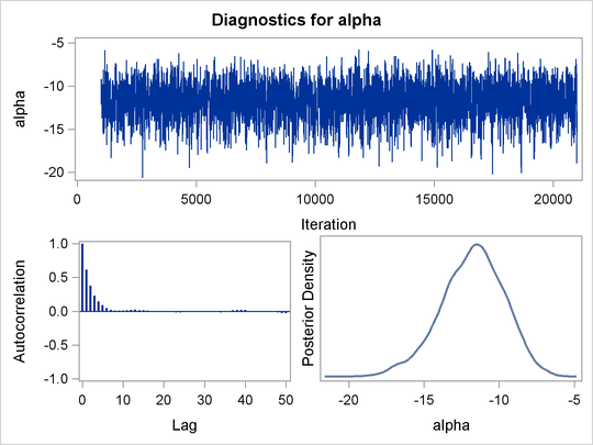
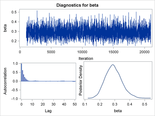
Trace plots and autocorrelation plots of the posterior samples are shown in Output 55.3.2. Convergence looks good in both parameters; there is good mixing in the trace plot and quick drop-off in the ACF plot.
One advantage of Bayesian methods is the ability to directly answer scientific questions. In this example, you might want
to find out the posterior probability that the environmental contaminant increases the probability of death—that is, ![]() . This can be estimated using the following steps:
. This can be estimated using the following steps:
proc format;
   value betafmt low-0 = 'beta <= 0' 0<-high = 'beta > 0';
run;

proc freq data=beetleout;
   tables beta /nocum;
   format beta betafmt.;
run;
Output 55.3.3: Frequency Counts
| Logistic Regression Model with a Diffuse Prior |
| beta | Frequency | Percent |
|---|---|---|
| beta > 0 | 10000 | 100.00 |
All of the simulated values for ![]() are greater than zero, so the sample estimate of the posterior probability that
are greater than zero, so the sample estimate of the posterior probability that ![]() is 100%. The evidence overwhelmingly supports the hypothesis that increased levels of the environmental contaminant increase
the probability of death.
is 100%. The evidence overwhelmingly supports the hypothesis that increased levels of the environmental contaminant increase
the probability of death.
If you are interested in making inference based on any quantities that are transformations of the random variables, you can
either do it directly in PROC MCMC or by using the DATA step after you run the simulation. Transformations sometimes can make
parameter inference quite formidable using direct analytical methods, but with simulated chains, it is easy to compute chains
for any set of parameters. Suppose you are interested in the lethal dose and want to estimate the level of the covariate x that corresponds to a probability of death, p. Abbreviate this quantity as ldp. In other words, you want to solve the logit transformation with a fixed value p. The lethal dose is as follows:
You can obtain an estimate of any ldp by using the posterior mean estimates for ![]() and
and ![]() . For example,
. For example, lp95, which corresponds to ![]() , is calculated as follows:
, is calculated as follows:
where –11.77 and 0.29 are the posterior mean estimates of ![]() and
and ![]() , respectively, and 50.79 is the estimated lethal dose that leads to a 95% death rate.
, respectively, and 50.79 is the estimated lethal dose that leads to a 95% death rate.
While it is easy to obtain the point estimates, it is harder to estimate other posterior quantities, such as the standard
deviation directly. However, with PROC MCMC, you can trivially get estimates of any posterior quantities of lp95. Consider the following program in PROC MCMC:
proc mcmc data=beetles ntu=1000 nmc=20000 nthin=2 propcov=quanew
          outpost=beetleout seed=246810 plot=density
          monitor=(pi30 ld05 ld50 ld95);
   ods select PostSummaries PostIntervals densitypanel;
   parms (alpha  beta) 0;
   begincnst;
      c1 = log(0.05 / 0.95);
      c2 = -c1;
   endcnst;

   beginnodata;
   prior alpha beta ~ normal(0, var = 10000);
   pi30 = logistic(alpha + beta*30);
   ld05 = (c1 - alpha) / beta;
   ld50 = - alpha / beta;
   ld95 = (c2 - alpha) / beta;
   endnodata;
   pi = logistic(alpha + beta*x);
   model y ~ binomial(n,pi);
run;
ods graphics off;
The program estimates four additional posterior quantities. The three lpd quantities, ld05, ld50, and ld95, are the three levels of the covariate that kills 5%, 50%, and 95% of the population, respectively. The predicted probability
when the covariate x takes the value of 30 is pi30. The MONITOR= option selects the quantities of interest. The PLOTS= option selects kernel density plots as the only ODS graphical output, excluding the trace plot and autocorrelation plot.
Programming statements between the BEGINCNST and ENDCNST statements define two constants. These statements are executed once at the beginning of the simulation. The programming statements
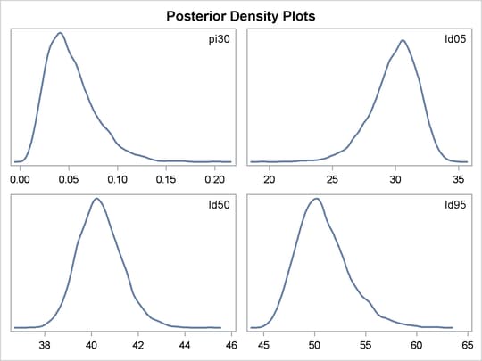
between the BEGINNODATA and ENDNODATA statements evaluate the quantities of interest. The symbols, pi30, ld05, ld50, and ld95, are functions of the parameters alpha and beta only. Hence, they should not be processed at the observation level and should be included in the BEGINNODATA and ENDNODATA statements. Output 55.3.4 lists the posterior summary and Output 55.3.5 shows the density plots of these posterior quantities.
Output 55.3.4: PROC MCMC Results
| Logistic Regression Model with a Diffuse Prior |
| Posterior Summaries | ||||||
|---|---|---|---|---|---|---|
| Parameter | N | Mean | Standard Deviation |
Percentiles | ||
| 25% | 50% | 75% | ||||
| pi30 | 10000 | 0.0524 | 0.0253 | 0.0340 | 0.0477 | 0.0662 |
| ld05 | 10000 | 29.9281 | 1.8814 | 28.8430 | 30.1727 | 31.2563 |
| ld50 | 10000 | 40.3745 | 0.9377 | 39.7271 | 40.3165 | 40.9612 |
| ld95 | 10000 | 50.8210 | 2.5353 | 49.0372 | 50.5157 | 52.3100 |
| Posterior Intervals | |||||
|---|---|---|---|---|---|
| Parameter | Alpha | Equal-Tail Interval | HPD Interval | ||
| pi30 | 0.050 | 0.0161 | 0.1133 | 0.0109 | 0.1008 |
| ld05 | 0.050 | 25.6409 | 32.9660 | 26.2193 | 33.2774 |
| ld50 | 0.050 | 38.6706 | 42.3718 | 38.6194 | 42.2811 |
| ld95 | 0.050 | 46.7180 | 56.7667 | 46.3221 | 55.8774 |
The posterior mean estimate of lp95 is 50.82, which is close to the estimate of 50.79 by using the posterior mean estimates of the parameters. With PROC MCMC,
in addition to the mean estimate, you can get the standard deviation, quantiles, and interval estimates at any level of significance.
From the density plots, you can see, for example, that the sample distribution for ![]() is skewed to the right, and almost all of your posterior belief concerning
is skewed to the right, and almost all of your posterior belief concerning ![]() is concentrated in the region between zero and 0.15.
is concentrated in the region between zero and 0.15.
It is easy to use the DATA step to calculate these quantities of interest. The following DATA step uses the simulated values
of ![]() and
and ![]() to create simulated values from the posterior distributions of
to create simulated values from the posterior distributions of ld05, ld50, ld95, and ![]() :
:
data transout;
   set beetleout;
   pi30 = logistic(alpha + beta*30);
   ld05 = (log(0.05 / 0.95) - alpha) / beta;
   ld50 = (log(0.50 / 0.50) - alpha) / beta;
   ld95 = (log(0.95 / 0.05) - alpha) / beta;
run;
Subsequently, you can use SAS/INSIGHT, or the UNIVARIATE, CAPABILITY, or KDE procedures to analyze the posterior sample. If you want to regenerate the default ODS graphs from PROC MCMC, see Regenerating Diagnostics Plots.