The GLM Procedure
-
Overview

-
Getting Started
-
Syntax
-
DetailsStatistical Assumptions for Using PROC GLMSpecification of EffectsUsing PROC GLM InteractivelyParameterization of PROC GLM ModelsHypothesis Testing in PROC GLMEffect Size Measures for F Tests in GLMAbsorptionSpecification of ESTIMATE ExpressionsComparing GroupsMultivariate Analysis of VarianceRepeated Measures Analysis of VarianceRandom-Effects AnalysisMissing ValuesComputational ResourcesComputational MethodOutput Data SetsDisplayed OutputODS Table NamesODS Graphics
-
ExamplesRandomized Complete Blocks with Means Comparisons and ContrastsRegression with Mileage DataUnbalanced ANOVA for Two-Way Design with InteractionAnalysis of CovarianceThree-Way Analysis of Variance with ContrastsMultivariate Analysis of VarianceRepeated Measures Analysis of VarianceMixed Model Analysis of Variance with the RANDOM StatementAnalyzing a Doubly Multivariate Repeated Measures DesignTesting for Equal Group VariancesAnalysis of a Screening Design
- References
This example demonstrates how you can test for equal group variances in a one-way design. The data come from the University of Pennsylvania Smell Identification Test (UPSIT), reported in O’Brien and Heft (1995). The study is undertaken to explore how age and gender are related to sense of smell. A total of 180 subjects 20 to 89 years old are exposed to 40 different odors: for each odor, subjects are asked to choose which of four words best describes the odor. The Freeman-Tukey modified arcsine transformation (Bishop, Fienberg, and Holland, 1975) is applied to the proportion of correctly identified odors to arrive at an olfactory index. For the following analysis, subjects are divided into five age groups:
|
|
|
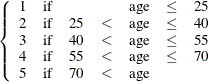 |
The following statements create a data set named upsit, containing the age group and olfactory index for each subject.
data upsit;
   input agegroup smell @@;
   datalines;
1 1.381  1 1.322  1 1.162  1 1.275  1 1.381  1 1.275  1 1.322
1 1.492  1 1.322  1 1.381  1 1.162  1 1.013  1 1.322  1 1.322
1 1.275  1 1.492  1 1.322  1 1.322  1 1.492  1 1.322  1 1.381
1 1.234  1 1.162  1 1.381  1 1.381  1 1.381  1 1.322  1 1.381
1 1.322  1 1.381  1 1.275  1 1.492  1 1.275  1 1.322  1 1.275
1 1.381  1 1.234  1 1.105
2 1.234  2 1.234  2 1.381  2 1.322  2 1.492  2 1.234  2 1.381
2 1.381  2 1.492  2 1.492  2 1.275  2 1.492  2 1.381  2 1.492
2 1.322  2 1.275  2 1.275  2 1.275  2 1.322  2 1.492  2 1.381
2 1.322  2 1.492  2 1.196  2 1.322  2 1.275  2 1.234  2 1.322
2 1.098  2 1.322  2 1.381  2 1.275  2 1.492  2 1.492  2 1.381
2 1.196
3 1.381  3 1.381  3 1.492  3 1.492  3 1.492  3 1.098  3 1.492
3 1.381  3 1.234  3 1.234  3 1.129  3 1.069  3 1.234  3 1.322
3 1.275  3 1.230  3 1.234  3 1.234  3 1.322  3 1.322  3 1.381
4 1.322  4 1.381  4 1.381  4 1.322  4 1.234  4 1.234  4 1.234
4 1.381  4 1.322  4 1.275  4 1.275  4 1.492  4 1.234  4 1.098
4 1.322  4 1.129  4 0.687  4 1.322  4 1.322  4 1.234  4 1.129
4 1.492  4 0.810  4 1.234  4 1.381  4 1.040  4 1.381  4 1.381
4 1.129  4 1.492  4 1.129  4 1.098  4 1.275  4 1.322  4 1.234
4 1.196  4 1.234  4 0.585  4 0.785  4 1.275  4 1.322  4 0.712
4 0.810
5 1.322  5 1.234  5 1.381  5 1.275  5 1.275  5 1.322  5 1.162
5 0.909  5 0.502  5 1.234  5 1.322  5 1.196  5 0.859  5 1.196
5 1.381  5 1.322  5 1.234  5 1.275  5 1.162  5 1.162  5 0.585
5 1.013  5 0.960  5 0.662  5 1.129  5 0.531  5 1.162  5 0.737
5 1.098  5 1.162  5 1.040  5 0.558  5 0.960  5 1.098  5 0.884
5 1.162  5 1.098  5 0.859  5 1.275  5 1.162  5 0.785  5 0.859
;
Older people are more at risk for problems with their sense of smell, and this should be reflected in significant differences in the mean of the olfactory index across the different age groups. However, many older people also have an excellent sense of smell, which implies that the older age groups should have greater variability. In order to test this hypothesis and to compute a one-way ANOVA for the olfactory index that is robust to the possibility of unequal group variances, you can use the HOVTEST and WELCH options in the MEANS statement for the GLM procedure, as shown in the following statements.
proc glm data=upsit;
   class agegroup;
   model smell = agegroup;
   means agegroup / hovtest welch;
run;
Output 42.10.1, Output 42.10.2, and Output 42.10.3 display the usual ANOVA test for equal age group means, Levene’s test for equal age group variances, and Welch’s test for equal age group means, respectively. The hypotheses of age effects for mean and variance of the olfactory index are both confirmed.
Output 42.10.1: Usual ANOVA Test for Age Group Differences in Mean Olfactory Index
| Source | DF | Type III SS | Mean Square | F Value | Pr > F |
|---|---|---|---|---|---|
| agegroup | 4 | 2.13878141 | 0.53469535 | 16.65 | <.0001 |
Output 42.10.2: Levene’s Test for Age Group Differences in Olfactory Variability
| Levene's Test for Homogeneity of smell Variance ANOVA of Squared Deviations from Group Means |
|||||
|---|---|---|---|---|---|
| Source | DF | Sum of Squares | Mean Square | F Value | Pr > F |
| agegroup | 4 | 0.0799 | 0.0200 | 6.35 | <.0001 |
| Error | 175 | 0.5503 | 0.00314 | ||
Output 42.10.3: Welch’s Test for Age Group Differences in Mean Olfactory Index
| Welch's ANOVA for smell | |||
|---|---|---|---|
| Source | DF | F Value | Pr > F |
| agegroup | 4.0000 | 13.72 | <.0001 |
| Error | 78.7489 | ||
As discussed in Homogeneity of Variance in One-Way Models, Levene’s test or any other test for homogeneity of variance should not be used as a diagnostic for the assumption of equal group variances that underlies the usual analysis of variance. However, graphical diagnostics can be a useful informal tool for monitoring whether your data meet the assumptions of a GLM analysis. The following statements perform a one-way ANOVA as before, but with ODS Graphics enabled. In addition to the box plot that is produced by default, the PLOTS=DIAGNOSTICS option requests a panel of summary diagnostics for the fit. These additional plots are shown in Output 42.10.4 and Output 42.10.5.
ods graphics on;
proc glm data=upsit plot=diagnostics;
   class agegroup;
   model smell = agegroup;
run;
ods graphics off;
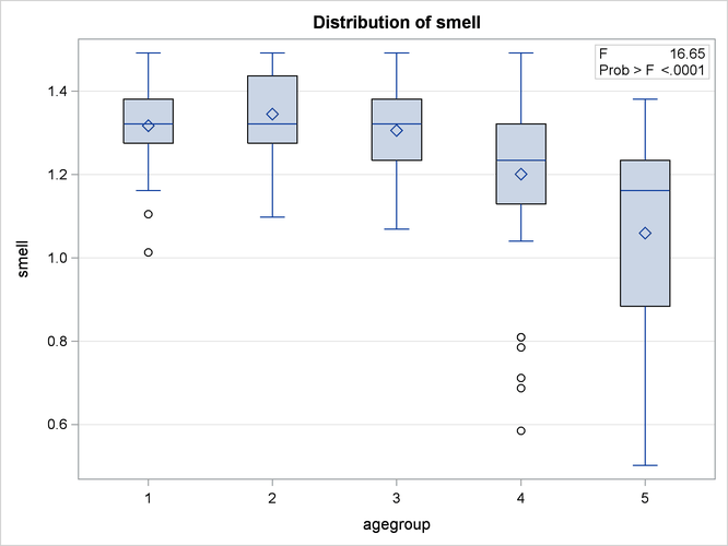
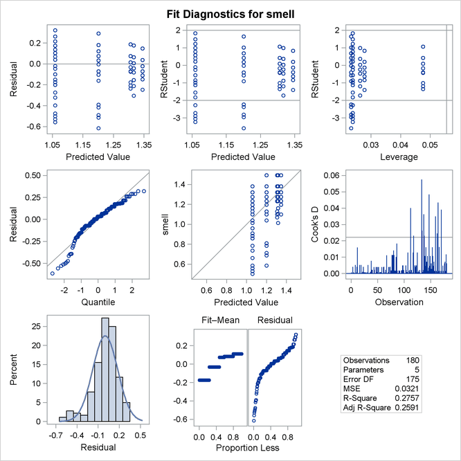
Output 42.10.4 clearly shows different degrees of variability for olfactory index within different age groups, with the variability generally rising with age. Likewise, several of the plots in the diagnostics panel shown in Output 42.10.5 indicate a relationship between olfactory variability and mean olfactory index. Also, note that the plot of Cook’s D statistic indicates that observations in the higher, more variable age groups are overly influential on the analysis of group means. The overall inference from these plots is that an assumption of equal group variances is probably untenable and that the analysis of the group means should thus take this into account.